Allowing the lower asymptote parameter to vary freely

Introduction

There may be situations where we want to estimate the lower asymptote of $h_0$ freely in our model rather than assuming it always starts at zero, which is what sicegar assumes by default. For this purpose, the functions fitAndCategorize() and figureModelCurves() contain the argument use_h0 (which has a default value set to FALSE). Setting the argument to TRUE results in the same process as usual, using functions ending in _h0 instead of their default counterparts. For example, the functions multipleFitFunction(), doublesigmoidalFitFormula(), parameterCalculation(), and normalizeData() have _h0 counterparts, multipleFitFunction_h0(), doublesigmoidalFitFormula_h0(), parameterCalculation_h0(), and normalizeData_h0().

We will demonstrate the differences between letting $h_0$ be estimated freely and assuming it is fixed at zero, first generating data where $h_0$ is not zero:

time <- seq(1, 24, 0.5)
noise_parameter <- 0.2
intensity_noise <- runif(n = length(time), min = 0, max = 1) * noise_parameter
intensity <- doublesigmoidalFitFormula_h0(time,
                                       finalAsymptoteIntensityRatio = .3,
                                       maximum = 10,
                                       slope1Param = 1,
                                       midPoint1Param = 7,
                                       slope2Param = 1,
                                       midPointDistanceParam = 8,
                                       h0 = 2)
intensity <- intensity + intensity_noise
dataInput <- data.frame(time, intensity)
ggplot(dataInput, aes(time, intensity)) + 
  geom_point() + 
  scale_y_continuous(limits = c(0, 12), expand = expansion(mult = c(0, 0))) + 
  theme_bw()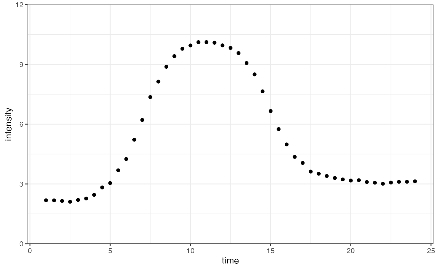

Fitting the models to the data

fitAndCategorize() can be applied to the data, first with default arguments and second by setting the argument use_h0 to TRUE:

fitObj_zero <- fitAndCategorize(dataInput,
                           threshold_minimum_for_intensity_maximum = 0.3,
                           threshold_intensity_range = 0.1,
                           threshold_t0_max_int = 0.05,
                           use_h0 = FALSE)   # Default

fitObj_free <- fitAndCategorize(dataInput,
                           threshold_minimum_for_intensity_maximum = 0.3,
                           threshold_intensity_range = 0.1,
                           threshold_t0_max_int = 0.05,
                           use_h0 = TRUE)

Using figureModelCurves(), we can visualize the differences between using the default arguments and letting $h_0$ be freely estimated.

# Double-sigmoidal fit with parameter related lines
fig_a <- figureModelCurves(dataInput = fitObj_zero$normalizedInput,
                                  doubleSigmoidalFitVector = fitObj_zero$doubleSigmoidalModel,
                                  showParameterRelatedLines = TRUE,
                                  use_h0 = FALSE)   # Default

## Warning: `aes_()` was deprecated in ggplot2 3.0.0.
## ℹ Please use tidy evaluation idioms with `aes()`
## ℹ The deprecated feature was likely used in the sicegar package.
##   Please report the issue at <https://hardin47.github.io/sicegar/issues>.
## This warning is displayed once every 8 hours.
## Call `lifecycle::last_lifecycle_warnings()` to see where this warning was
## generated.

## Warning: Using `size` aesthetic for lines was deprecated in ggplot2 3.4.0.
## ℹ Please use `linewidth` instead.
## ℹ The deprecated feature was likely used in the sicegar package.
##   Please report the issue at <https://hardin47.github.io/sicegar/issues>.
## This warning is displayed once every 8 hours.
## Call `lifecycle::last_lifecycle_warnings()` to see where this warning was
## generated.

fig_b <- figureModelCurves(dataInput = fitObj_free$normalizedInput,
                                  doubleSigmoidalFitVector = fitObj_free$doubleSigmoidalModel,
                                  showParameterRelatedLines = TRUE,
                                  use_h0 = TRUE)

plot_grid(fig_a, fig_b, ncol = 2) # function from the cowplot package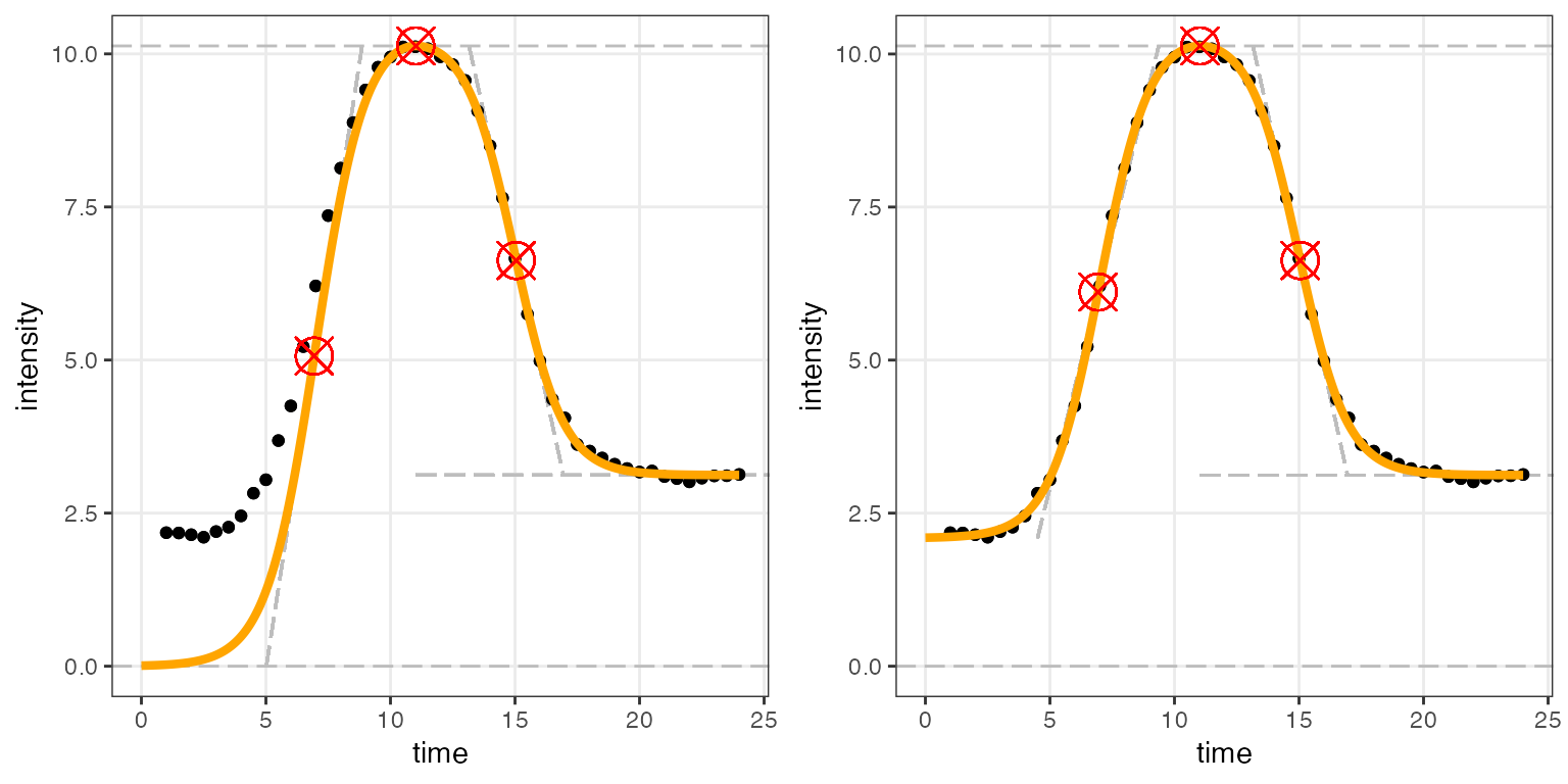

It is clear that in this situation, using the default arguments result in a worse fit than when $h_0$ is allowed to be estimated freely.

Model fitting components ( $h_0$ free)

To fit and plot individual models using a freely estimated $h_0$ , we must directly call the _h0 counterparts of each sicegar function. We have already generated the data (with $h_0 = 2$ ), so now we can normalize the data.

normalizedInput_free <- normalizeData(dataInput = dataInput, 
                                 dataInputName = "doubleSigmoidalSample")
head(normalizedInput_free$timeIntensityData) # the normalized time and intensity data

##         time   intensity
## 1 0.04166667 0.009226536
## 2 0.06250000 0.008663863
## 3 0.08333333 0.005118997
## 4 0.10416667 0.000000000
## 5 0.12500000 0.011497350
## 6 0.14583333 0.020499679

We can now call multipleFitFunction_h0() on our data to be fitted, calculating additional parameters using parameterCalculation_h0():

# Fit the double-sigmoidal model
doubleSigmoidalModel_free <- multipleFitFunction_h0(dataInput=normalizedInput_free,
                                            model="doublesigmoidal")

doubleSigmoidalModel_free <- parameterCalculation_h0(doubleSigmoidalModel_free)

Now that we have obtained a fit, we can use figureModelCurves() to plot:

# double-sigmoidal fit
figureModelCurves(dataInput = normalizedInput_free,
                  doubleSigmoidalFitVector = doubleSigmoidalModel_free,
                  showParameterRelatedLines = TRUE,
                  use_h0 = TRUE)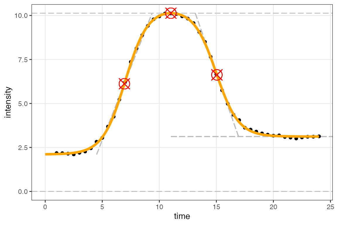

Model parameters

Recall that the original model parameters (which generated the data) are given as finalAsymptoteIntensityRatio = 0.3, maximum = 10, slope1Param = 1, midPoint1Param = 7, slope2Param = 1, midPointDistanceParam = 8, h0 = 2.

We can recover the parameter estimates from both of the doubleSigmoidalModel objects created above. fitObj_zero does not return a value for $h_0$ (because it is not part of the estimation process). The rest of the parameter values are nearly identical, but models with $h_0 = 0$ are fundamentally different from models with $h_0 \ne 0$ .

fitObj_zero$doubleSigmoidalModel |>
  select(finalAsymptoteIntensityRatio_Estimate, maximum_Estimate, slope1Param_Estimate, midPoint1Param_Estimate,
         slope2Param_Estimate, midPointDistanceParam_Estimate) |> 
  c()

## $finalAsymptoteIntensityRatio_Estimate
## [1] 0.3080899
## 
## $maximum_Estimate
## [1] 10.13
## 
## $slope1Param_Estimate
## [1] 1.007482
## 
## $midPoint1Param_Estimate
## [1] 7.006687
## 
## $slope2Param_Estimate
## [1] 1.021521
## 
## $midPointDistanceParam_Estimate
## [1] 7.976228

fitObj_free$doubleSigmoidalModel |>
  select(finalAsymptoteIntensityRatio_Estimate, maximum_Estimate, slope1Param_Estimate, midPoint1Param_Estimate,
         slope2Param_Estimate, midPointDistanceParam_Estimate, h0_Estimate) |> c()

## $finalAsymptoteIntensityRatio_Estimate
## [1] 0.3079927
## 
## $maximum_Estimate
## [1] 10.13192
## 
## $slope1Param_Estimate
## [1] 1.001984
## 
## $midPoint1Param_Estimate
## [1] 7.003664
## 
## $slope2Param_Estimate
## [1] 1.020129
## 
## $midPointDistanceParam_Estimate
## [1] 7.97747
## 
## $h0_Estimate
## [1] 2.091675

Thomas Matheis, Phineus Choi, Sam Butler, Mira Terdiman, Jo Hardin

2025-10-03

Introduction

Fitting the models to the data

Model fitting components ( $h_0$ free)

Model parameters

Allowing the lower asymptote parameter to vary freely

Thomas Matheis, Phineus Choi, Sam Butler, Mira Terdiman, Jo Hardin

2025-10-03

Introduction

Fitting the models to the data

Model fitting components (h0h_0 free)

Model parameters

Model fitting components ( $h_0$ free)