Sigmoidal fit function with h0 estimation

The function fits a sigmoidal curve to given data by using likelihood maximization (LM) algorithm and provides the parameters (maximum, slopeParam, midPoint, and h0) describing the double-sigmoidal fit as output. It also contains information about the goodness of fits such as AIC, BIC, residual sum of squares, and log likelihood.

Usage

sigmoidalFitFunction_h0(
  dataInput,
  tryCounter,
  startList = list(maximum = 1, slopeParam = 1, midPoint = 0.33, h0 = 0),
  lowerBounds = c(maximum = 0.3, slopeParam = 0.01, midPoint = -0.52, h0 = -0.1),
  upperBounds = c(maximum = 1.5, slopeParam = 180, midPoint = 1.15, h0 = 0.3),
  min_Factor = 1/2^20,
  n_iterations = 1000
)

Arguments

dataInput

A data frame or a list containing the dataframe. The data frame should be composed of at least two columns. One represents time, and the other represents intensity. The data should be normalized with the normalize data function sicegar::normalizeData() before imported into this function.

tryCounter

A counter that shows the number of times the data was fit via maximum likelihood function.

startList

A vector containing the initial set of parameters that the algorithm tries for the first fit attempt for the relevant parameters. The vector composes of four elements; 'maximum', 'slopeParam', 'midPoint', and 'h0'. Detailed explanations of those parameters can be found in vignettes. Defaults are maximum = 1, slopeParam = 1, midPoint = 0.33, and h0 = 0. The numbers are in normalized time intensity scale.

lowerBounds

The lower bounds for the randomly generated start parameters. The vector composes of four elements; 'maximum', 'slopeParam', 'midPoint', and 'h0'. Detailed explanations of those parameters can be found in vignettes. Defaults are maximum = 0.3, slopeParam = 0.01, midPoint = -0.52, and h0 = -0.1. The numbers are in normalized time intensity scale.

upperBounds

The upper bounds for the randomly generated start parameters. The vector composes of four elements; 'maximum', 'slopeParam','midPoint', and 'h0'. Detailed explanations of those parameters can be found in vignettes. Defaults are maximum = 1.5, slopeParam = 180, midPoint = 1.15, and h0 = 0.3. The numbers are in normalized time intensity scale.

min_Factor

Defines the minimum step size used by the fitting algorithm. Default is 1/2^20.

n_iterations

Defines maximum number of iterations used by the fitting algorithm. Default is 1000

Value

Returns fitted parameters for the sigmoidal model.

Examples

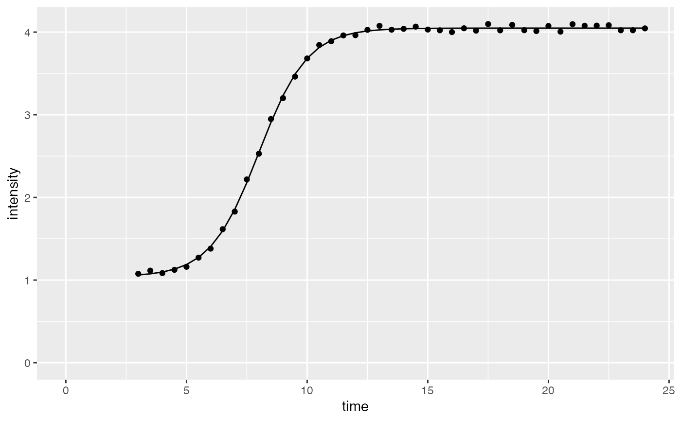
time <- seq(3, 24, 0.5)

#simulate intensity data and add noise
noise_parameter <- 0.1
intensity_noise <- stats::runif(n = length(time), min = 0, max = 1) * noise_parameter
intensity <- sigmoidalFitFormula_h0(time, maximum = 4, slopeParam = 1, midPoint = 8, h0 = 1)
intensity <- intensity + intensity_noise

dataInput <- data.frame(intensity = intensity, time = time)
normalizedInput <- normalizeData(dataInput)
parameterVector <- sigmoidalFitFunction_h0(normalizedInput, tryCounter = 1)

#Check the results
# sigmoidalFitFunction_h0() is run on the startList param values (because 'tryCounter = 1')
# use multipleFitFunction() for multiple random starts in order to optimize
if(parameterVector$isThisaFit){
intensityTheoretical <- sigmoidalFitFormula_h0(time,
                                           maximum = parameterVector$maximum_Estimate,
                                           slopeParam = parameterVector$slopeParam_Estimate,
                                           midPoint = parameterVector$midPoint_Estimate,
                                           h0 = parameterVector$h0_Estimate)

comparisonData <- cbind(dataInput, intensityTheoretical)

require(ggplot2)
ggplot(comparisonData) +
 geom_point(aes(x = time, y = intensity)) +
 geom_line(aes(x = time, y = intensityTheoretical)) +
 expand_limits(x = 0, y = 0)
}


if(!parameterVector$isThisaFit){
  print(parameterVector)
}