Introduction

The overarching aim of this package is to fit both a sigmoidal and a double-sigmoidal curve to time–intensity data and then determine which of the two models fit the data best. The sigmoidal model is assumed to start at zero and rise to an asymptotic value. The double-sigmoidal model first increases from 0 to a maximum intensity and the decreases to a final asymptotic intensity. For both the sigmoid and double-sigmoid models, we provide an option to let the lower asymptote ( $h_0$ ) freely vary. After calculating the best candidate curves for both of models a decision algorithm determines which of the two candidates (if any) fits the data best. Finally, the package calculates key parameters that quantify the time–intensity data with respect to the best-fitting model.

For the sigmoidal model, key parameters describing the curve are:

maximum: The maximum asymptotic intensity.
midpoint: The time point at which the sigmoidal curve reaches half of its maximum intensity.
slope: The slope of the curve at the midpoint.

For the double-sigmoidal model, key parameters describing the curve are:

maximum: The maximum intensity the double-sigmoidal curve reaches.
final asymptotic intensity: The intensity the curve decreases to after having reached its maximum.
midpoint 1: The time point at which the double-sigmoidal curve reaches half of its maximum intensity during the initial rise.
slope 1: The slope at midpoint 1.
midpoint 2: The time point at which the double-sigmoidal curve reaches the intensity corresponding to the mean of the maximum intensity and the final asymptotic intensity.
slope 2: The slope at midpoint 2.

Importantly, the parameters used to mathematically describe the fitted curves do not necessarily directly correspond to these intuitively meaningful parameters. Therefore, the sicegar package calculates the intuitively meaningful parameters from the estimated parameters. See the vignette on additional parameters for details.

Example fit on simulated input data

The input to the fitting function must be in the form of a data frame with two columns called time and intensity. We will here use double-sigmoidal data generated with some arbitrarily chosen parameters. We can use the function doublesigmoidalFitFormula() to generate a double-sigmoidal curve, to which we add random noise.

time <- seq(3, 24, 0.5)
noise_parameter <- 0.2
intensity_noise <- runif(n = length(time), min = 0, max = 1) * noise_parameter
intensity <- doublesigmoidalFitFormula(time,
                                    finalAsymptoteIntensityRatio = .3,
                                    maximum = 4,
                                    slope1Param = 1,
                                    midPoint1Param = 7,
                                    slope2Param = 1,
                                    midPointDistanceParam = 8)
intensity <- intensity+intensity_noise
dataInput <- data.frame(time, intensity)

ggplot(dataInput, aes(time, intensity)) + geom_point() + theme_bw()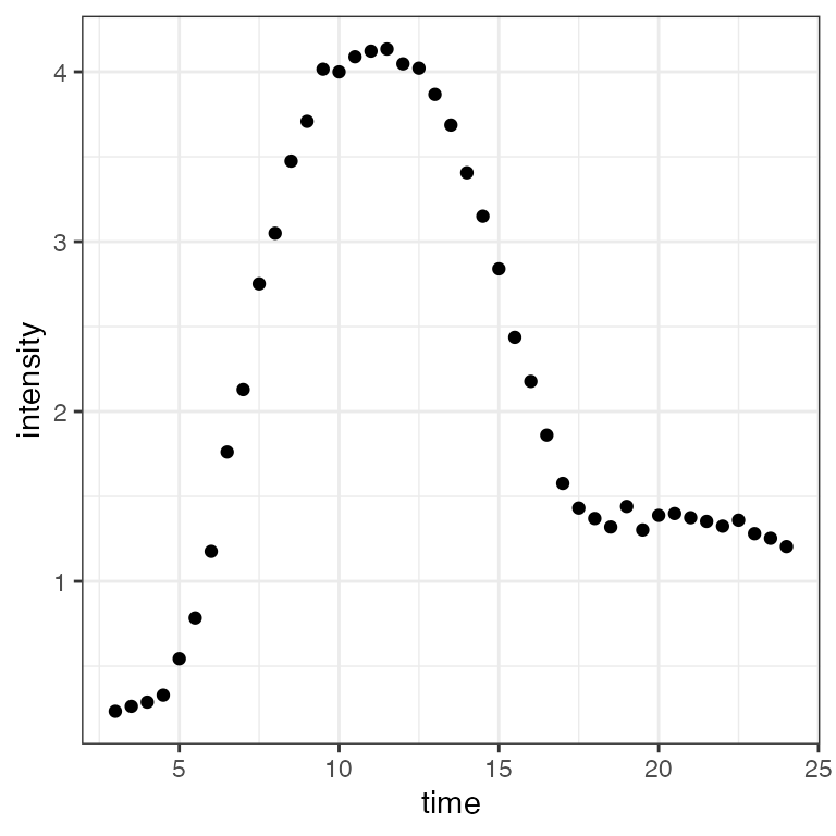

We can now fit the two models to the data and determine which is the better fit. This is done with the function fitAndCategorize(). The three provided threshold parameters are used in the categorization process and depend on the units in which the data are measured. See the vignette on categorizing fits for details.

fitObj <- fitAndCategorize(dataInput,
                           threshold_minimum_for_intensity_maximum = 0.3,
                           threshold_intensity_range = 0.1,
                           threshold_t0_max_int = 1E10)

The two fitted curves can be visualized with the function figureModelCurves(), which returns a ggplot2 plot.

# Double-sigmoidal fit with parameter related lines
fig_a <- figureModelCurves(dataInput = fitObj$normalizedInput,
                                  sigmoidalFitVector = fitObj$sigmoidalModel,
                                  showParameterRelatedLines = TRUE)

## Warning: `aes_()` was deprecated in ggplot2 3.0.0.
## ℹ Please use tidy evaluation idioms with `aes()`
## ℹ The deprecated feature was likely used in the sicegar package.
##   Please report the issue at <https://hardin47.github.io/sicegar/issues>.
## This warning is displayed once every 8 hours.
## Call `lifecycle::last_lifecycle_warnings()` to see where this warning was
## generated.

## Warning: Using `size` aesthetic for lines was deprecated in ggplot2 3.4.0.
## ℹ Please use `linewidth` instead.
## ℹ The deprecated feature was likely used in the sicegar package.
##   Please report the issue at <https://hardin47.github.io/sicegar/issues>.
## This warning is displayed once every 8 hours.
## Call `lifecycle::last_lifecycle_warnings()` to see where this warning was
## generated.

fig_b <- figureModelCurves(dataInput = fitObj$normalizedInput,
                                  doubleSigmoidalFitVector = fitObj$doubleSigmoidalModel,
                                  showParameterRelatedLines = TRUE)

plot_grid(fig_a, fig_b, ncol = 2) # function from the cowplot package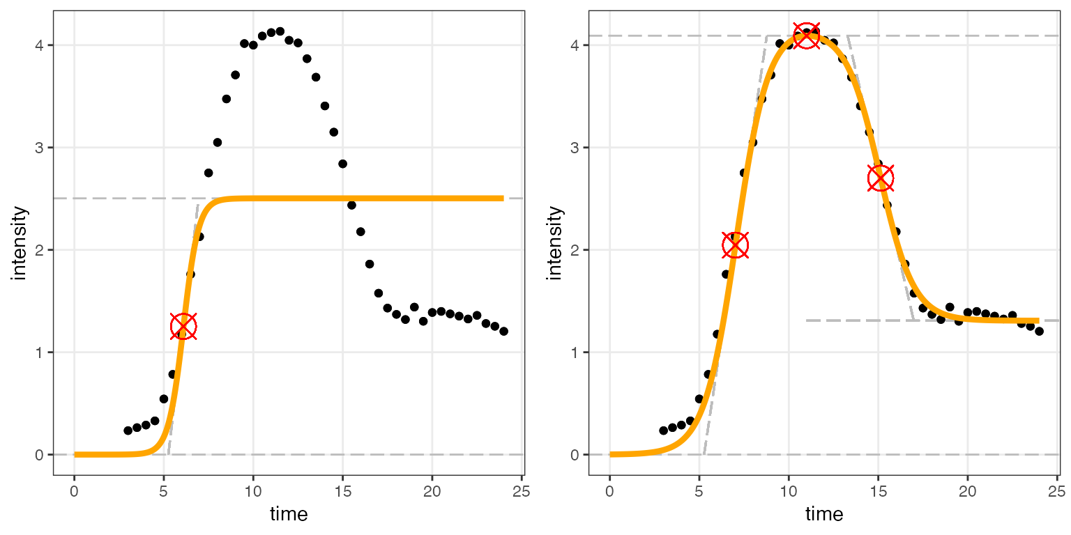

Clearly the regular sigmoidal curve does not provide a good fit but the double-sigmoidal curve does. This information is available from the returned fit object:

fitObj$decisionProcess$decision # final decision

## [1] "double_sigmoidal"

The fit object

The fit object returned by fitAndCategorize() contains all the information potentially of interest in the course of this type of an analysis. It consists of five distinct components:

names(fitObj)

## [1] "normalizedInput"      "sigmoidalModel"       "doubleSigmoidalModel"
## [4] "decisionProcess"      "summaryVector"

Each component holds numerous parameters of interest:

.$normalizedInput: The normalized dataset with normalization parameters, so that the raw dataset can be recovered from the normalized one. For more information, see the vignette on fitting individual models.
.$sigmoidalModel: The parameters for the sigmoidal fit. For more information, see the vignettes on fitting individual models and on additional parameters.
.$doubleSigmoidalModel: The parameters for the double-sigmoidal fit. For more information, see the vignettes on fitting individual models and on additional parameters.
.$decisionProcess: The results from the decision process of which of the two models fit the data better. For more information, see the vignette on categorizing fits.
.$summaryVector: Key parameters of the winning model. These are the most important parameters extracted from either .$sigmoidalModel or .$doubleSigmoidalModel.

Here, the contents of the summary vector is as follows:

str(fitObj$summaryVector)

## List of 21
##  $ dataInputName          : logi NA
##  $ decision               : chr "double_sigmoidal"
##  $ maximum_x              : num 11
##  $ maximum_y              : num 4.09
##  $ midPoint1_x            : num 7.02
##  $ midPoint1_y            : num 2.05
##  $ midPoint2_x            : num 15.1
##  $ midPoint2_y            : num 2.7
##  $ slope1                 : num 1.17
##  $ slope2                 : num -0.754
##  $ finalAsymptoteIntensity: num 1.31
##  $ incrementTime          : num 3.51
##  $ startPoint_x           : num 5.27
##  $ startPoint_y           : num 0
##  $ reachMaximum_x         : num 8.77
##  $ reachMaximum_y         : num 4.09
##  $ decrementTime          : num 3.69
##  $ startDeclinePoint_x    : num 13.3
##  $ startDeclinePoint_y    : num 4.09
##  $ endDeclinePoint_x      : num 17
##  $ endDeclinePoint_y      : num 1.31

All these parameters are defined in the vignette on additional parameters.

Umut Caglar, Claus O. Wilke

2025-10-03

Example fit on simulated input data

The fit object