Adjusting data to use with sicegar

Thomas Matheis, Phineus Choi, Sam Butler, Mira Terdiman, Johanna Hardin

2025-11-15

Adjusting the data structure

There are sometimes cases where data must be adjusted before using sicegar. Two common situations in which adjustments are needed is when the data have too few time points and when there appears to be a decreasing, or negative, trend. While sicegar does not have built-in functions to perform the necessary corrections, we provide a set of straightforward operations to mitigate the cases and estimate the sigmoidal parameter values.

Too few time points / observations

The first case happens when the data contain too few time points. More specifically, if the sigmoidal data has on the order of five or fewer time points (six or fewer for double sigmoidal data), sicegar will usually fail to find a fit. This is a result of the sigmoidal and double sigmoidal models having six and seven parameters respectively.

time <- rep(seq(1, 24, 4), 5)
noise_parameter <- 0.3
mean_values <- doublesigmoidalFitFormula_h0(time,
                                       finalAsymptoteIntensityRatio = .3,
                                       maximum = 10,
                                       slope1Param = 1,
                                       midPoint1Param = 7,
                                       slope2Param = 1,
                                       midPointDistanceParam = 8,
                                       h0 = 3)
intensity <- rnorm(n = length(mean_values), mean = mean_values, sd = rep(noise_parameter, length(mean_values)))

dataInput <- data.frame(time, intensity)
ggplot(dataInput, aes(time, intensity)) + 
  geom_point() + 
  scale_y_continuous(limits = c(0, 12), expand = expansion(mult = c(0, 0))) + 
  theme_bw()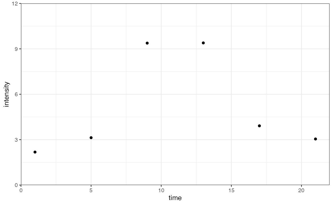

We can attempt to use fitAndCategorize() on our data, only to observe that the function fails to find a fit and results in an error:

fitObj <- fitAndCategorize(dataInput,
                           threshold_minimum_for_intensity_maximum = 0.3,
                           threshold_intensity_range = 0.1,
                           threshold_t0_max_int = 1E10,
                           use_h0 = TRUE)

## Error in if (parameterVector$model == "sigmoidal") {: argument is of length zero

When there are multiple reps at each time point, a small jitter in the x-direction (time) can artificially “create more time points” for the sicegar estimation.

dataInput_jitter <- dataInput |>
  mutate(time = jitter(time, amount = 0.5))
  
ggplot(dataInput_jitter, aes(time, intensity)) + 
  geom_point() + 
  scale_y_continuous(limits = c(0, 12), expand = expansion(mult = c(0, 0))) + 
  theme_bw()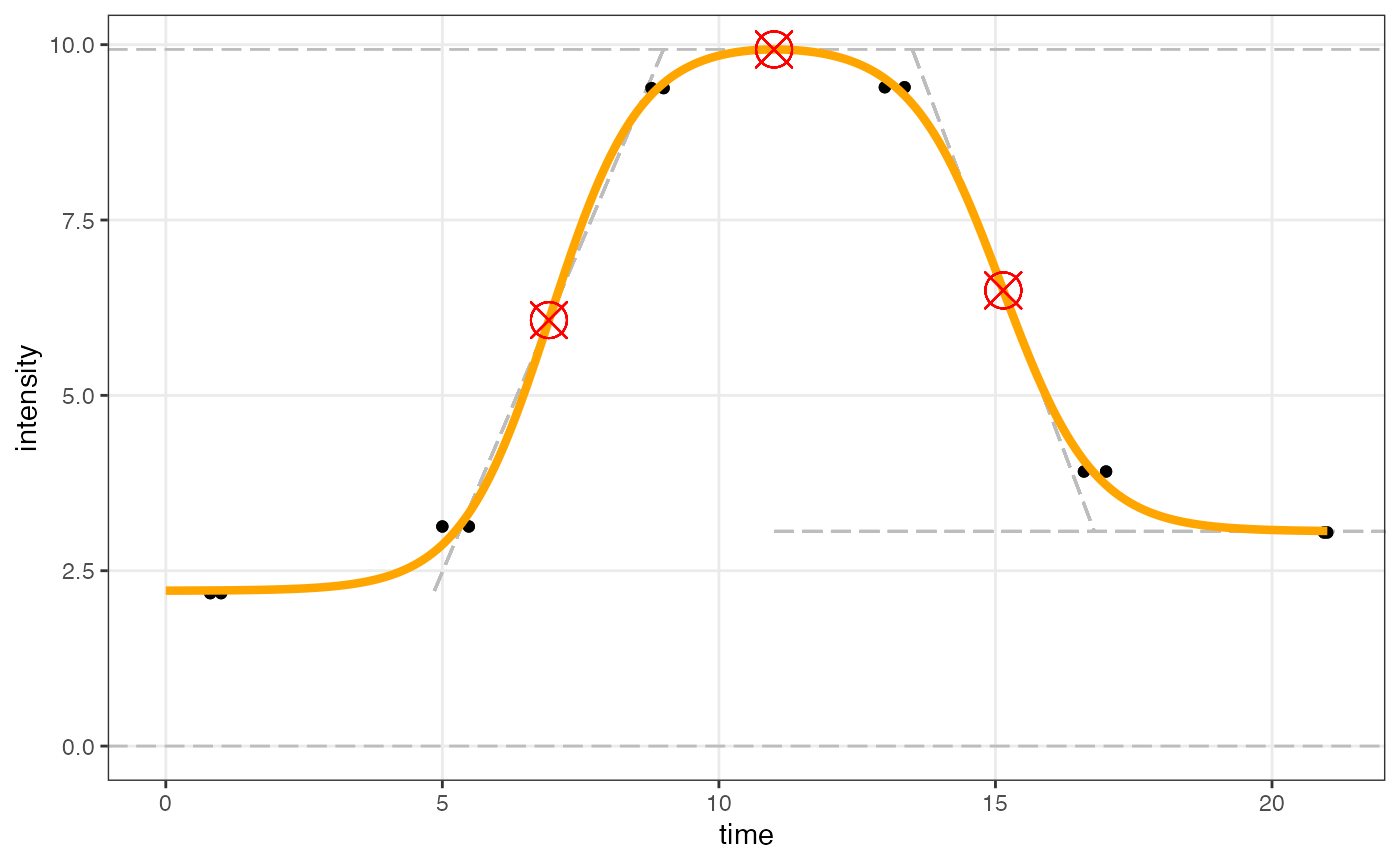

fitAndCategorize is used as usual, successfully finding a fit for the model. Data are plotted using figureModelCurves():

fitObj_jittered <- fitAndCategorize(dataInput_jitter,
                           threshold_minimum_for_intensity_maximum = 0.3,
                           threshold_intensity_range = 0.1,
                           threshold_t0_max_int = 1E10,
                           use_h0 = TRUE)

figureModelCurves(dataInput = fitObj_jittered$normalizedInput,
                  doubleSigmoidalFitVector = fitObj_jittered$doubleSigmoidalModel,
                  showParameterRelatedLines = TRUE,
                  use_h0 = TRUE)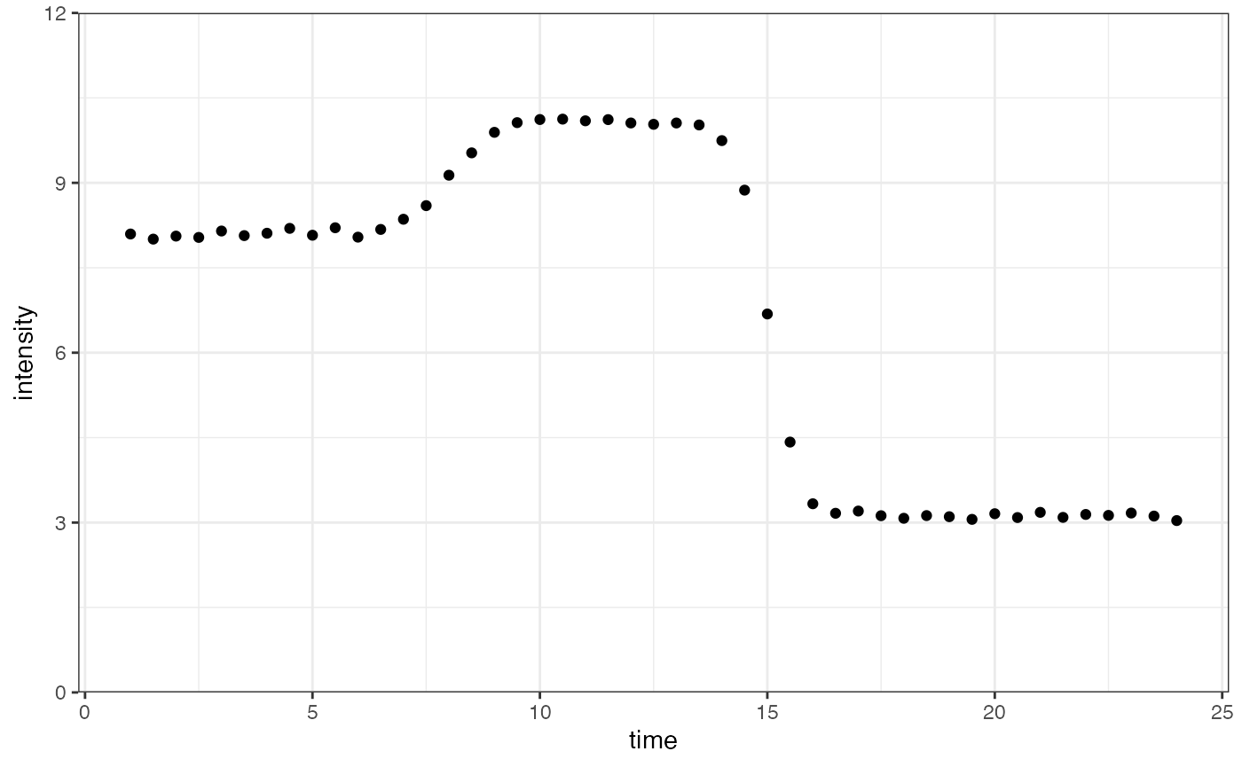

Decreasing trend

The second case happens when there is a negative relationship between time and intensity. The solution is to reverse the time points (subtract time from max(time)) and fit the model in the flipped space. Then flip the model back (e.g., the $t1$ parameter can be estimated in the flipped space and then unflipped to get the original onset time).

time <- seq(1, 24, 0.5)
noise_parameter <- 0.2
mean_values <- doublesigmoidalFitFormula_h0(time,
                                       finalAsymptoteIntensityRatio = .3,
                                       maximum = 10,
                                       slope1Param = 1,
                                       midPoint1Param = 7,
                                       slope2Param = 1,
                                       midPointDistanceParam = 8,
                                       h0 = 8)
intensity <- rnorm(n = length(mean_values), mean = mean_values, sd = rep(noise_parameter, length(mean_values)))

dataInput <- data.frame(time, intensity)
ggplot(dataInput, aes(time, intensity)) + 
  geom_point() + 
  scale_y_continuous(limits = c(0, 12), expand = expansion(mult = c(0, 0))) + 
  theme_bw()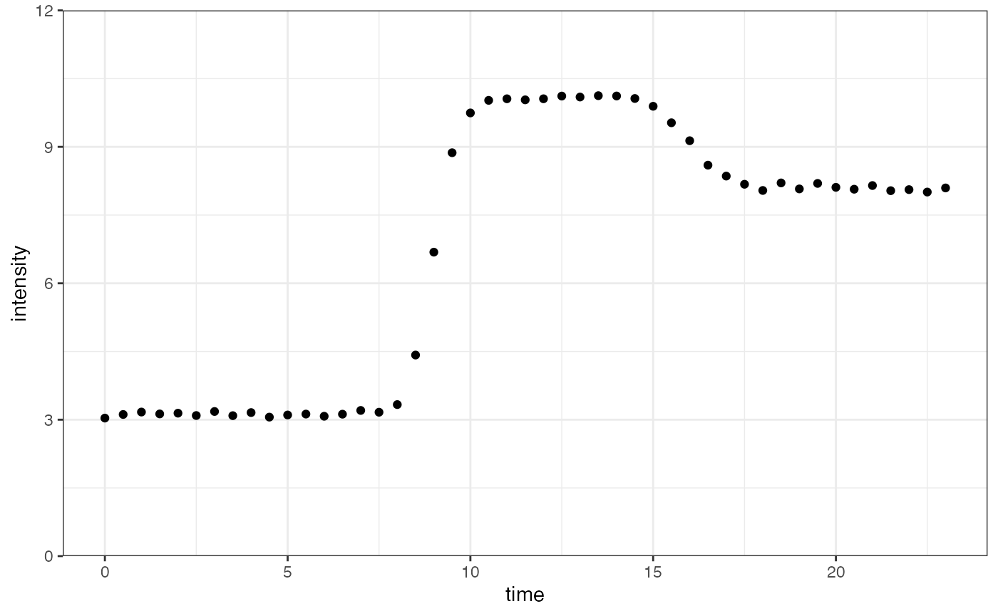

The most straightforward method to deal with decreasing trends is to reverse the x-axis, resulting in the last time value to becoming the first time value, etc. The new time is calculated as max(time) - time.

dataInput_flipped <- dataInput |>
  mutate(time = max(time) - time)

ggplot(dataInput_flipped, aes(time, intensity)) + 
  geom_point() + 
  scale_y_continuous(limits = c(0, 12), expand = expansion(mult = c(0, 0))) + 
  theme_bw()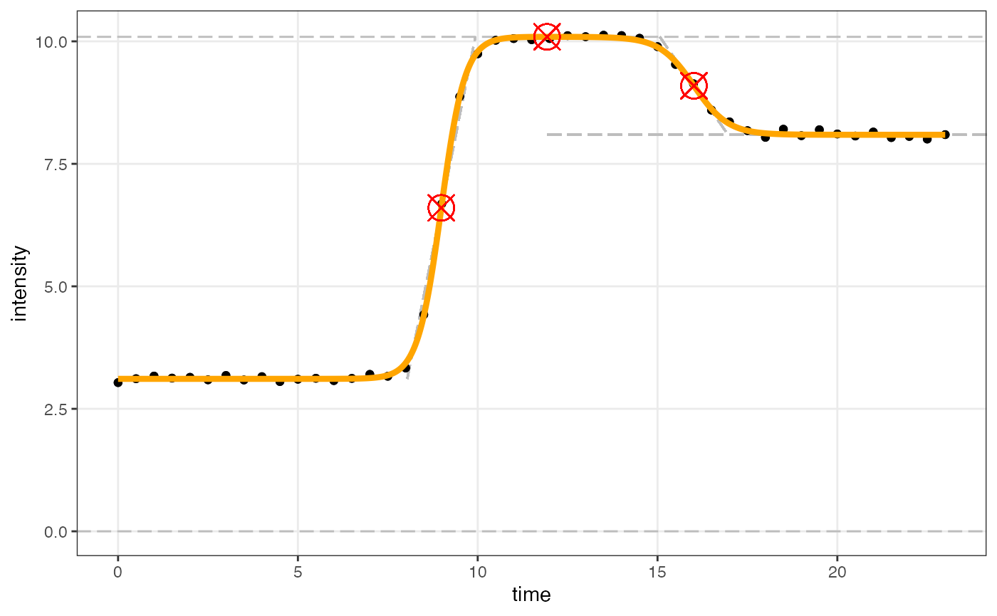

Now that the data have an increasing trend, we can apply fitAndCategorize as usual to find a fit for our model and plot using figureModelCurves():

fitObj_flipped <- fitAndCategorize(dataInput_flipped,
                           threshold_minimum_for_intensity_maximum = 0.3,
                           threshold_intensity_range = 0.1,
                           threshold_t0_max_int = 1E10,
                           use_h0 = TRUE)

figureModelCurves(dataInput = fitObj_flipped$normalizedInput,
                  doubleSigmoidalFitVector = fitObj_flipped$doubleSigmoidalModel,
                  showParameterRelatedLines = TRUE,
                  use_h0 = TRUE)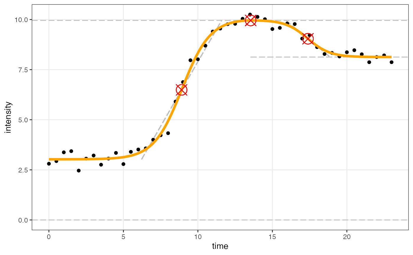

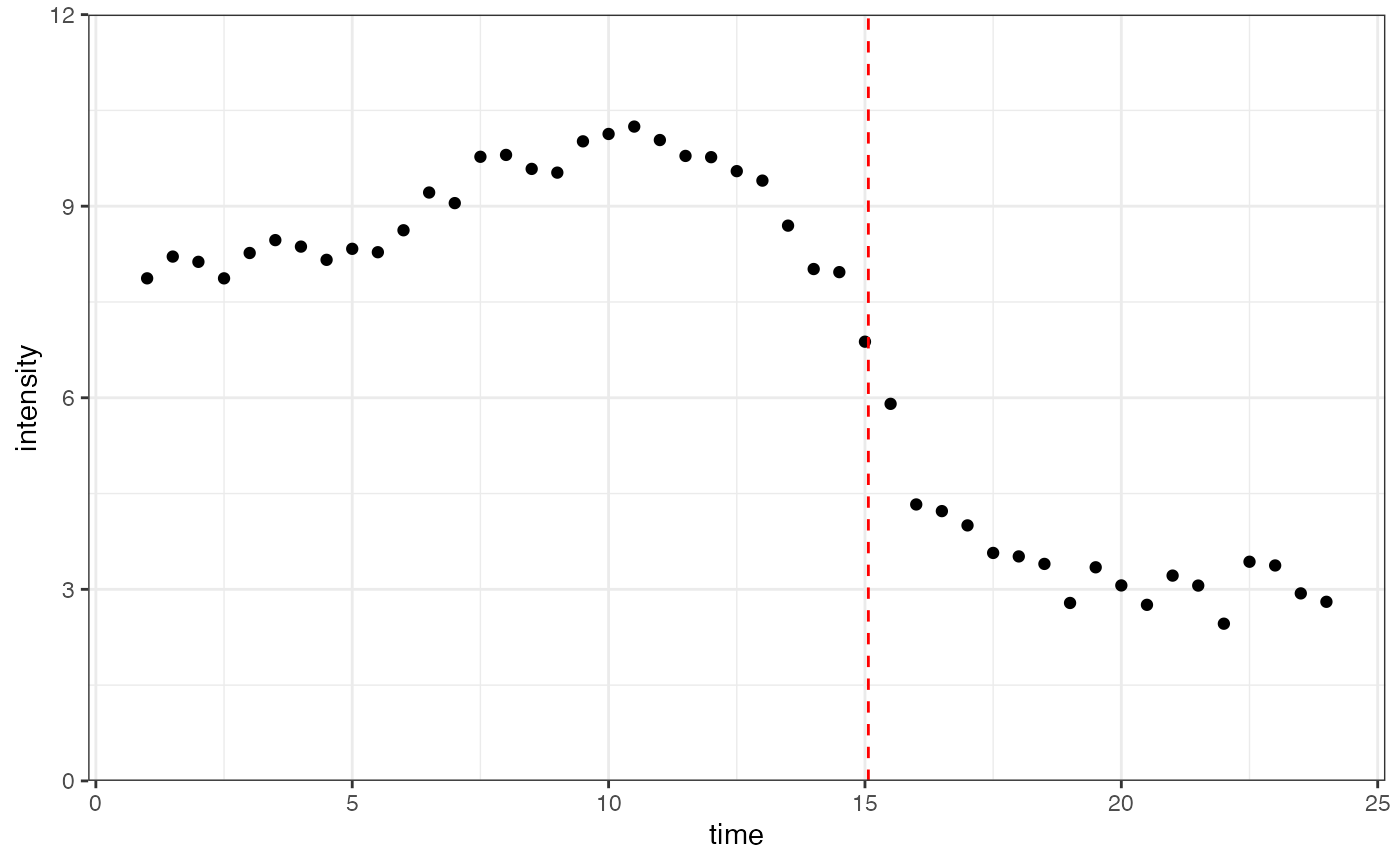
To extract the original onset time, we convert the $t1$ parameter back to the original space, observing the final estimation on the original data:

original_onset_time <- max(dataInput$time) - fitObj_flipped$doubleSigmoidalModel$midPoint1Param_Estimate

dataInput <- data.frame(time, intensity)
ggplot(dataInput, aes(time, intensity)) + 
  geom_point() + 
  geom_vline(xintercept = original_onset_time, color = "red", linetype = "dashed") +
  scale_y_continuous(limits = c(0, 12), expand = expansion(mult = c(0, 0))) + 
  theme_bw()