Henley Passport Index Data

library(tidyverse) # ggplot, lubridate, dplyr, stringr, readr...
library(praise)
library(jsonlite)
library(plotly)
library(sf)
library(rnaturalearth)
library(rnaturalearthdata)

The Data

This week we are exploring data from the Henley Passport Index API. The Henley Passport Index is produced by Henley & Partners and captures the number of countries to which travelers in possession of each passport in the world may enter visa free.

country_lists <- readr::read_csv('https://raw.githubusercontent.com/rfordatascience/tidytuesday/main/data/2025/2025-09-09/country_lists.csv')
rank_by_year <- readr::read_csv('https://raw.githubusercontent.com/rfordatascience/tidytuesday/main/data/2025/2025-09-09/rank_by_year.csv')

travel_perms <- country_lists |> 
  janitor::clean_names() %>%
  setNames(gsub("_", " ", names(.))) |> 
  pivot_longer(
    cols = c(`visa required`, `visa online`, `visa on arrival`, 
             `visa free access`, `electronic travel authorisation`),
    names_to = "visa_type",
    values_to = "json_str"
 ) |> 
  mutate(
    json_parsed = map(json_str, ~ fromJSON(.)[[1]])
) |> 
  unnest(json_parsed, names_sep = "_") |> 
  select(-json_str) |> 
  rename(from = code, from_name = country,
         to = json_parsed_code, to_name = json_parsed_name) |> 
  mutate(from = ifelse(from_name == "Namibia", "NA", from)) 
 #mutate(visa_type = case_when(
 #  visa_type == "visa_required" ~ "visa_required",
 #  visa_type == "visa_online" ~ "visa_required",
 #  visa_type == "visa_on_arrival" ~ "visa_required",
 #  visa_type == "visa_free_access" ~ "easy_access",
 #  visa_type == "electronic_travel_authorisation" ~ "easy_access"
 #)) |> 
 #  distinct()

travel_perms

# A tibble: 44,973 × 5
   from  from_name             visa_type     to    to_name    
   <chr> <chr>                 <chr>         <chr> <chr>      
 1 PS    Palestinian Territory visa required AF    Afghanistan
 2 PS    Palestinian Territory visa required DZ    Algeria    
 3 PS    Palestinian Territory visa required AD    Andorra    
 4 PS    Palestinian Territory visa required AO    Angola     
 5 PS    Palestinian Territory visa required AI    Anguilla   
 6 PS    Palestinian Territory visa required AR    Argentina  
 7 PS    Palestinian Territory visa required AM    Armenia    
 8 PS    Palestinian Territory visa required AW    Aruba      
 9 PS    Palestinian Territory visa required AT    Austria    
10 PS    Palestinian Territory visa required BB    Barbados   
# ℹ 44,963 more rows

Adding the home countries so that they show up on the map.

home_countries <- travel_perms |> 
  select(from, from_name) |> 
  distinct() |> 
  mutate(visa_type = "domestic",
         to = from,
         to_name = from_name)

travel_perms <- travel_perms |> rbind(home_countries)

Plotting

Would be great to have the plot be interactive so that the type of visa needed for travel is based on any country which is clicked on. Instead, we’ve created static map with information for Mexican travelers.

The interactive version of the plot (for any country’s travel restrictions) is too big for plotly. It could be done using a Shiny app.

world <- ne_countries(scale = "medium", returnclass = "sf")

world_data <- world |> 
  left_join(travel_perms, by = c("iso_a2_eh" = "to"))

world_data |> 
  filter(from == "MX") |> 
ggplot() +
  geom_sf(aes(fill = visa_type)) +
  theme_minimal() + 
  labs(title = "Visa connections for Mexicans",
       fill = "visa type")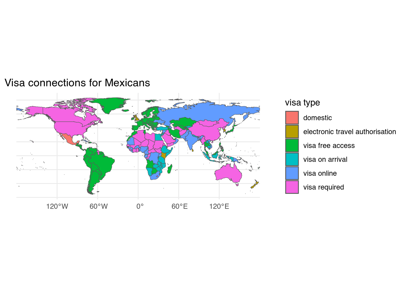

Each country is filled based on the type of visa needed for Mexican travelers. Note that Mexico is colored differently because domestic travel does not require a visa.

plot_ly() |> 
  add_sf(
    data = world_data |> filter(from == "MX"),
    split = ~iso_a2_eh,
    color = ~visa_type,
    text = ~paste0("Country: ", to_name, "<br>Visa: ", visa_type)#,
    #hoveron = "fills"
  ) |> 
  layout(title = "Visa connections for Mexicans",
         showlegend = FALSE)

Each country is filled based on the type of visa needed for Mexican travelers. Note that Mexico is colored differently because domestic travel does not require a visa.

praise()

[1] "You are priceless!"