Australian Frogs

library(tidyverse) # ggplot, lubridate, dplyr, stringr, readr...
library(praise)

The Data

This week we’re exploring 2023 data from the sixth annual release of FrogID data.

FrogID is an Australian frog call identification initiative. The FrogID mobile app allows citizen scientists to record and submit frog calls for museum experts to identify. Since 2017, FrogID data has contributed to over 30 scientific papers exploring frog ecology, taxonomy, and conservation.

Australia is home to a unique and diverse array of frog species found almost nowhere else on Earth, with 257 native species distributed throughout the continent. But Australia’s frogs are in peril – almost one in five species are threatened with extinction due to threats such as climate change, urbanisation, disease, and the spread of invasive species.

frogID_data <- readr::read_csv('https://raw.githubusercontent.com/rfordatascience/tidytuesday/main/data/2025/2025-09-02/frogID_data.csv') |> 
  mutate(month = month(eventDate),
         season = case_when(
           month %in% c(12, 1, 2) ~ "winter",
           month %in% c(3, 4, 5) ~ "spring",
           month %in% c(6, 7, 8) ~ "summer",
           month %in% c(9, 10, 11) ~ "fall"
         ))
frog_names <- readr::read_csv('https://raw.githubusercontent.com/rfordatascience/tidytuesday/main/data/2025/2025-09-02/frog_names.csv')

all_frogs <- frogID_data |>
  left_join(frog_names, by = "scientificName") |> 
  mutate(genus = stringr::str_extract(scientificName, "^\\w+"))

New color palette

library(Polychrome)

set.seed(47)
mycols <- createPalette(26, c("#ff0000", "#00ff00", "#0000ff"))

names(mycols) <- all_frogs |> select(genus) |> unique() |> pull()

A map

library(maps)
australia_map <- map(database = "world", region = "Australia",
                     plot = FALSE)

ggplot(data = australia_map, 
       aes(x = long, y = lat, group = group)) +
  geom_polygon(fill = "white", color = "blue") + 
  geom_point(data = all_frogs,
             aes(x = decimalLongitude, 
                 y = decimalLatitude, 
                 color = genus),
             size = 1,
             inherit.aes = FALSE) +
  theme_minimal() + 
  theme(
        panel.background = element_rect(fill = "lightsteelblue"), 
        panel.grid.major = element_line(color = "lightsteelblue"), 
        panel.grid.minor = element_line(color = "lightsteelblue2"), 
        axis.text = element_text(color = "black"),      
        axis.title = element_text(color = "black") ) +
  ggtitle("Frogs in Australia") + 
  facet_wrap(~season) + 
  labs(x = "", y = "") +
  scale_color_manual(values = mycols)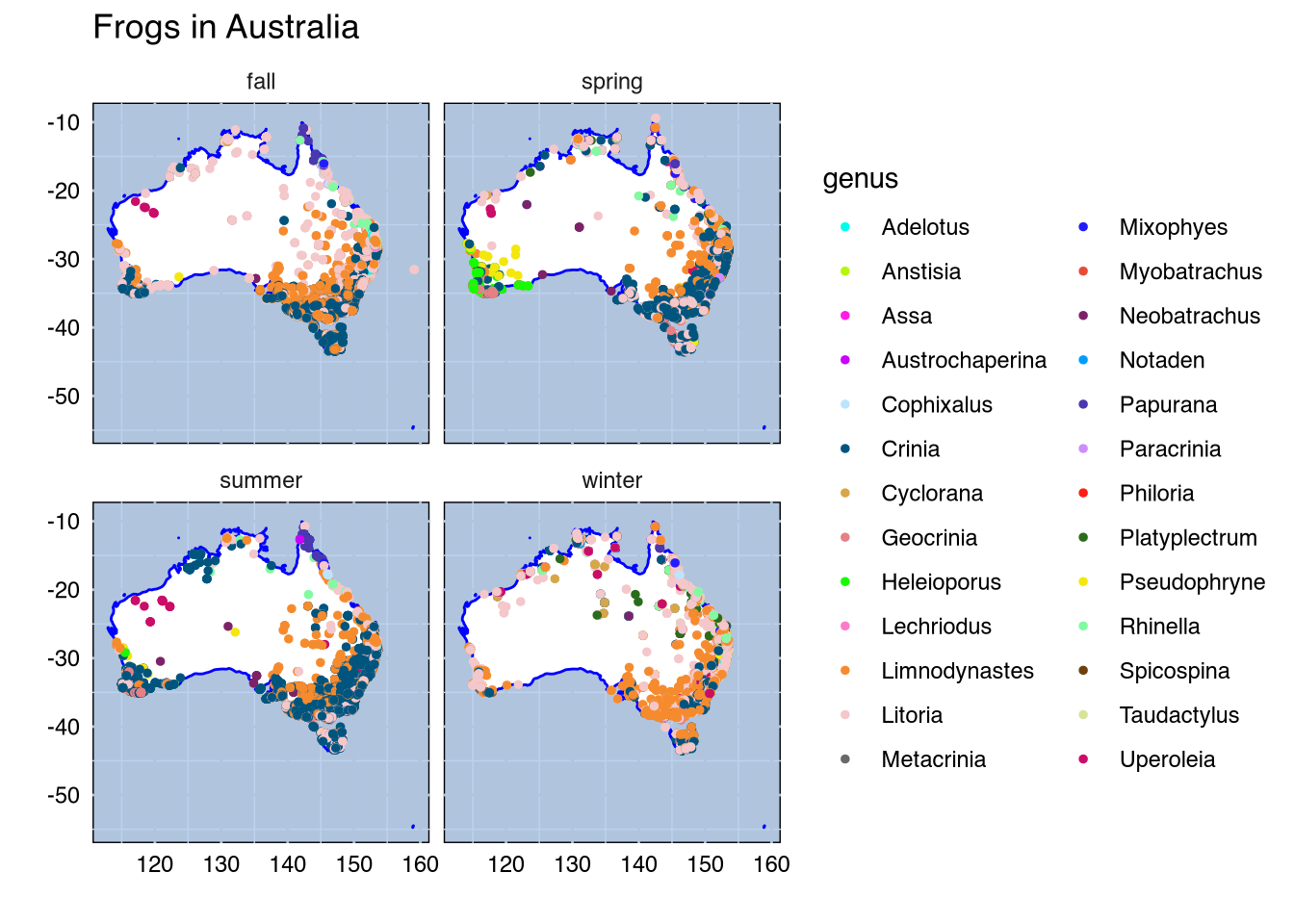

Citizen science observed frogs in Australia in 2023.

library(plotly)
p <- ggplot(data = australia_map, 
       aes(x = long, y = lat, group = group)) +
  geom_polygon(fill = "white", color = "blue") + 
  geom_point(data = all_frogs,
             aes(x = decimalLongitude, 
                 y = decimalLatitude, 
                 color = genus,
                 text = paste("common name:", commonName)),
             size = 1,
             inherit.aes = FALSE) +
  theme_minimal() + 
  theme(
        panel.background = element_rect(fill = "lightsteelblue"), 
        panel.grid.major = element_line(color = "lightsteelblue"), 
        panel.grid.minor = element_line(color = "lightsteelblue2"), 
        axis.text = element_text(color = "black"),      
        axis.title = element_text(color = "black") ) +
  ggtitle("Frogs in Australia") + 
  facet_wrap(~season) + 
  labs(x = "", y = "") +
  scale_color_manual(values = mycols)
  
  
ggplotly(p, tooltip = "genus") 

Citizen science observed frogs in Australia in 2023.

praise()

[1] "You are fantastic!"