Water Insecurity

The Data

This week we’re exploring water insecurity data featured in the article Mapping water insecurity in R with tidycensus!

Water insecurity can be influenced by number of social vulnerability indicators—from demographic characteristics to living conditions and socioeconomic status —that vary spatially across the U.S. This blog shows how the tidycensus package for R can be used to access U.S. Census Bureau data, including the American Community Surveys, as featured in the “Unequal Access to Water” data visualization from the USGS Vizlab. It offers reproducible code examples demonstrating use of tidycensus for easy exploration and visualization of social vulnerability indicators in the Western U.S.

The average household size was scraped from: https://worldpopulationreview.com/state-rankings/average-household-size-by-state

water_insecurity_2022 <- readr::read_csv('https://raw.githubusercontent.com/rfordatascience/tidytuesday/main/data/2025/2025-01-28/water_insecurity_2022.csv') |> 
  select(-geometry)
water_insecurity_2023 <- readr::read_csv('https://raw.githubusercontent.com/rfordatascience/tidytuesday/main/data/2025/2025-01-28/water_insecurity_2023.csv') |> 
  select(-geometry)

ave_household <- readr::read_csv("ave_household.csv")

Wrangling

Inspiration from @nrennie, https://github.com/nrennie/tidytuesday/tree/main/2025/2025-01-28.

We are looking to compare the percent of water insecurity in 2023 versus 2022, across states. According to the GitHub repository, the population is number of people and the plumbing variable is number of households. After summarizing the number of households over an entire state, we multiply by the average household size in that state (to get the number of people with water insecurity).

water_insec <- water_insecurity_2022 |> 
  inner_join(water_insecurity_2023, by = "geoid", suffix = c(".2022", ".2023")) |> 
  tidyr::separate(col = name.2022, into = c("city", "state"), sep = ", ") |> 
  select(-name.2023, -percent_lacking_plumbing.2022, -percent_lacking_plumbing.2023)


water_insec

# A tibble: 848 × 9
   geoid city             state year.2022 total_pop.2022 plumbing.2022 year.2023
   <chr> <chr>            <chr>     <dbl>          <dbl>         <dbl>     <dbl>
 1 01069 Houston County   Alab…      2022         108079            93      2023
 2 04001 Apache County    Ariz…      2022          65432          2440      2023
 3 06037 Los Angeles Cou… Cali…      2022        9721138          6195      2023
 4 06097 Sonoma County    Cali…      2022         482650           148      2023
 5 06001 Alameda County   Cali…      2022        1628997           808      2023
 6 06045 Mendocino County Cali…      2022          89783            18      2023
 7 08077 Mesa County      Colo…      2022         158636           128      2023
 8 06055 Napa County      Cali…      2022         134300             0      2023
 9 10005 Sussex County    Dela…      2022         255956           123      2023
10 12086 Miami-Dade Coun… Flor…      2022        2673837          1377      2023
# ℹ 838 more rows
# ℹ 2 more variables: total_pop.2023 <dbl>, plumbing.2023 <dbl>

diff_plumb <- water_insec |> 
  group_by(state) |> 
  summarize(total_2022 = sum(total_pop.2022, na.rm = TRUE),
         total_2023 = sum(total_pop.2023, na.rm = TRUE),
         no_plumb_2022 = sum(plumbing.2022, na.rm = TRUE),
         no_plumb_2023 = sum(plumbing.2023, na.rm = TRUE)) |> 
  full_join(ave_household, by = "state") |> 
  mutate(perc_no_plumb_2022 = 100*no_plumb_2022 * size / total_2022,
         perc_no_plumb_2023 = 100*no_plumb_2023 * size / total_2023,
         change_plumbing = perc_no_plumb_2023 - perc_no_plumb_2022)

data(state)
state_abbreviations <- data.frame(state.name, state.abb) |> 
  rbind(c("Puerto Rico", "PR")) |> 
  rbind(c("District of Columbia", "DC")) |> 
  mutate(state = as.factor(state.name))

Plotting

We plot both the difference (2023 minus 2022) in water insecurity as well as the proportion of the population with water insecurity in 2023.

diff_plumb |> 
  inner_join(state_abbreviations, by = "state") |>
  mutate(nudge = ifelse(change_plumbing > 0, 0.05, -0.05)) |> 
  ggplot(aes(x = change_plumbing, y = fct_reorder(state.abb, change_plumbing))) + 
  geom_col(aes(fill = change_plumbing)) + 
  geom_text(aes(label = fct_reorder(state.abb, change_plumbing), 
                x = change_plumbing + nudge), 
                size = 3) + 
  theme_minimal() + 
  theme(axis.text.y = element_blank(),
        panel.grid.major.y = element_blank()) + 
  labs(x = "Change in percent of population lacking plumbing between 2022 and 2023",
       y = "",
       fill = "difference in insecurity\n 2023 minus 2022") + 
  scale_fill_continuous(low = "blue", high = "orange")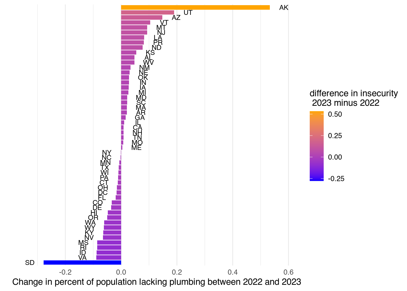

Bar plot with change in percent of population as water insecure from 2022 to 2023. The x-axis gives the difference in percentages 2023 minus 2022. Alaska had an additional 0.5% of its population as water insecure in 2023 as compared to 2022. South Dakota had a decrease of 0.3% of its population as water insecure in 2023 as compared to 2022. — For each state, we calculate the percentage of the population who is water insecure in both 2023 and 2022. The x-axis gives the difference in percentages 2023 minus 2022. Alaska had an additional 0.5% of its population as water insecure in 2023 as compared to 2022. South Dakota had a decrease of 0.3% of its population as water insecure in 2023 as compared to 2022.

diff_plumb |> 
  inner_join(state_abbreviations, by = "state") |>
  mutate(nudge = ifelse(change_plumbing > 0, 0.05, -0.05)) |> 
  ggplot(aes(x = perc_no_plumb_2023, y = fct_reorder(state.abb, change_plumbing))) + 
  geom_col(aes(fill = perc_no_plumb_2023)) + 
  geom_text(aes(label = fct_reorder(state.abb, change_plumbing), 
                x = perc_no_plumb_2023 + 0.05),
                size = 3) + 
  theme_minimal() + 
  theme(axis.text.y = element_blank(),
        panel.grid.major.y = element_blank()) + 
  labs(x = "Percent of population lacking plumbing in 2023",
       y = "",
       fill = "percent of insecurity 2023") + 
  scale_fill_continuous(low = "blue", high = "orange")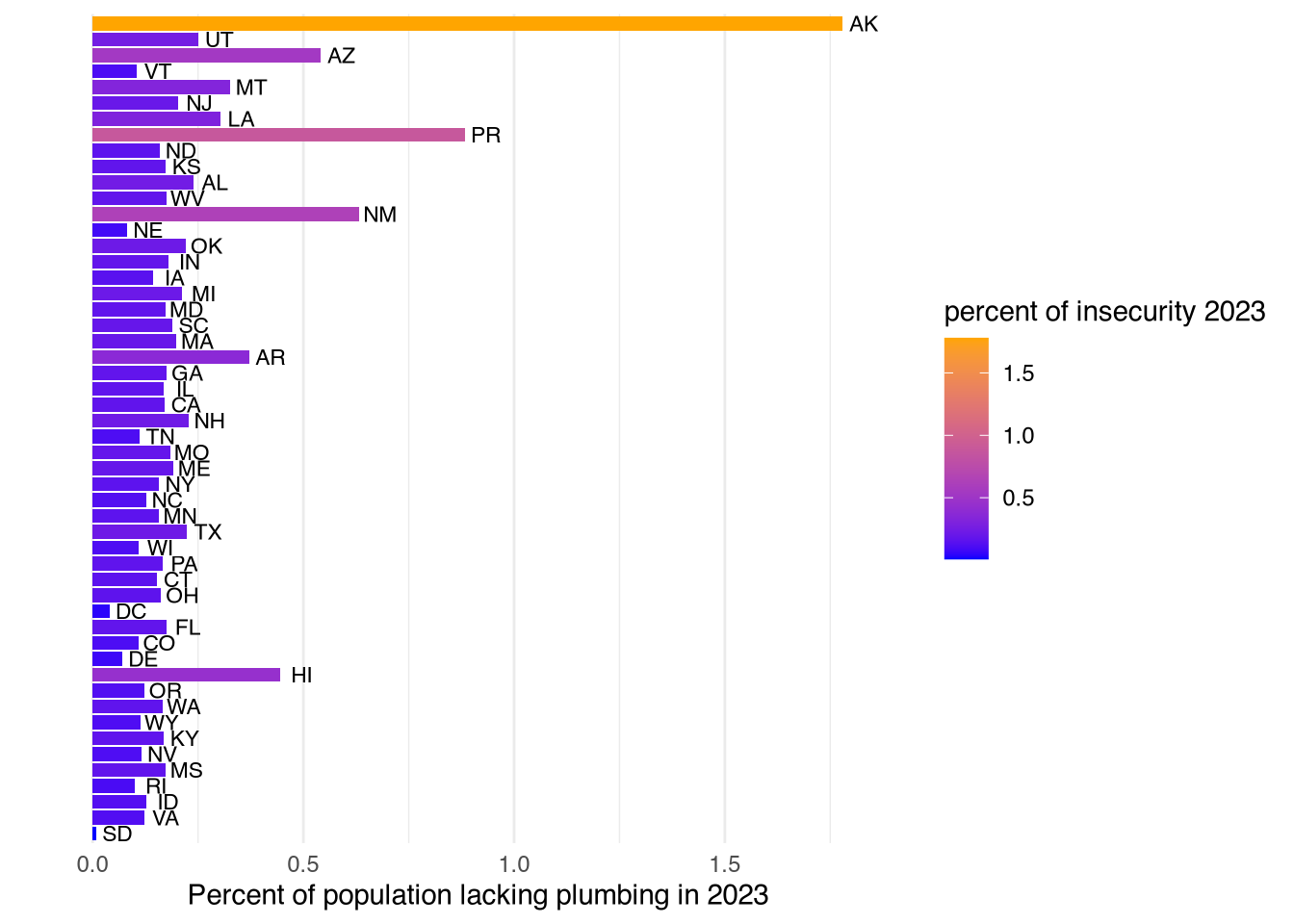

Bar plot with percent of population as water insecure on the x axis and state on the y axis. Alaska is the state with the highest percentage of the population as water insecure, at 1.3%. South Dakota is the state with the lowest percentage of the population as water insecure, at close to zero percent. — Note that while Alaska (approximately 1.3% of the population) and South Dakota (almost 0% of the population) are on the extremes of the percent of the population who is water insecure, the change from 2022 to 2023 does not monotonically match to the percentage of the state who is water insecure.

praise()

[1] "You are slick!"