library(tidyverse) # ggplot, lubridate, dplyr, stringr, readr...
library(praise)Himalayan Mountaineering Expeditions
The Data
This week, we are exploring mountaineering data from the Himalayan Dataset!
The Himalayan Database is a comprehensive archive documenting mountaineering expeditions in the Nepal Himalaya. It continues the pioneering work of Elizabeth Hawley, a journalist who dedicated much of her life to cataloging climbing history in the region. Her meticulous records were initially compiled from a wide range of sources, including books, alpine journals, and direct correspondence with Himalayan climbers.
exped_tidy <- readr::read_csv('https://raw.githubusercontent.com/rfordatascience/tidytuesday/main/data/2025/2025-01-21/exped_tidy.csv')
peaks_tidy <- readr::read_csv('https://raw.githubusercontent.com/rfordatascience/tidytuesday/main/data/2025/2025-01-21/peaks_tidy.csv')
Success?
Using the 882 expeditions, we calculate the success rate as a function of group size and mountain range. There is a slight positive trend in that larger groups seem more likely to succeed (where succeed is defined as success on at least one of the four routes pursued).
exped_tidy |>
  full_join(peaks_tidy, by = "PEAKID") |>
  filter(TOTMEMBERS > 0) |>
  mutate(total = TOTMEMBERS + TOTHIRED, deaths = MDEATHS + HDEATHS,
         prop_death = deaths / total,
         success = SUCCESS1 | SUCCESS2 | SUCCESS3 | SUCCESS4) |>
  mutate(total_factor = case_when(
    TOTMEMBERS <=  5 ~ 5,
    TOTMEMBERS <= 10 ~ 10,
    TOTMEMBERS <= 15 ~ 15,
    TOTMEMBERS <= 20 ~ 20,
    TRUE ~ 25
  )) |>
  group_by(total_factor, REGION_FACTOR) |>
  mutate(n_exped = n(), prop_success = mean(success)) |>
  ggplot(aes(x = total_factor, y = prop_success, color = REGION_FACTOR)) +
  geom_point(aes(size = n_exped), alpha = 0.5) +
  geom_line() +
  facet_wrap( ~ REGION_FACTOR) +
  labs(x = "Team size (number of members)",
       y = "proportion of teams who succeeded",
       size = "number of\nexpeditions") +
  scale_colour_discrete(guide = "none")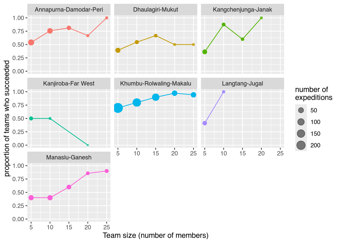
praise()[1] "You are wondrous!"