Monster Movies

Author

Jo Hardin

Published

October 29, 2024

library(tidyverse) # ggplot, lubridate, dplyr, stringr, readr...
library(ggmosaic)
library(tidymodels)
library(rpart.plot)
library(praise)

The Data

This week we’re exploring “monster” movies: movies with “monster” in their title!

The data this week comes from the Internet Movie Database. Check out “Why Do People Like Horror Films? A Statistical Analysis” for an exploration of “the unique appeal of scary movies”.

Along with importing the data, we one-hot encode the genres into their own binary variables (for modeling later).

monster_movie_genres <- readr::read_csv('https://raw.githubusercontent.com/rfordatascience/tidytuesday/master/data/2024/2024-10-29/monster_movie_genres.csv')
monster_movies <- readr::read_csv('https://raw.githubusercontent.com/rfordatascience/tidytuesday/master/data/2024/2024-10-29/monster_movies.csv') |> 
  separate_rows(genres, sep = ",") |> 
  mutate(value = 1) |> 
  pivot_wider(names_from = genres, values_from = value, values_fill = 0)

Viz

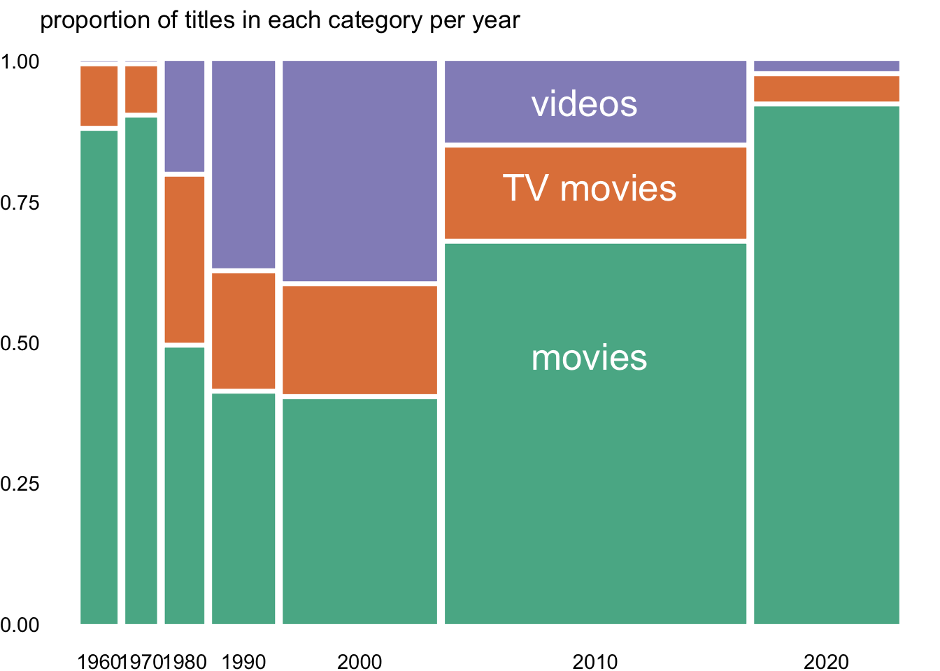
Taking inspiration from @stevenponce, we create a mosaic plot of the types of films over the last 60 years.

maybe change the font to spooky …

plot_data <- monster_movies |>
    mutate(title_type = str_to_title(title_type)) |> 
    mutate(decade = floor(year / 10) * 10) |> 
    filter(decade >= 1960) |> 
    drop_na(title_type, decade) |>
    count(title_type, decade) 

plot_data |> 
  ggplot() + 
  geom_mosaic(aes(weight = n, x = product(decade),
                  fill = title_type)) + 
  theme_void() + 
  labs(title = "proportion of titles in each category per year") + 
  theme(axis.text.x = element_text(),
        axis.text.y = element_text(),
        legend.position = "none") + 
  scale_y_continuous() +
  annotate(
        "text",
        x = .55, y = .5, label = "movies",
        color = "white", size = 7, vjust = 1, hjust = 0
    ) +
    annotate(
        "text",
        x = .515, y = .8, label = "TV movies",
        color = "white", size = 7, vjust = 1, hjust = 0
    ) +
    annotate(
        "text",
        x = .55, y = .95, label = "videos",
        color = "white", size = 7, vjust = 1, hjust = 0
    ) + 
  scale_fill_brewer(palette = "Dark2")

A mosaic plot showing the proportion of monster movies has changed over decades.

Model

Let’s try to predict the average IMDb rating! The first model we’ll choose is a linear model. The genres have been re-coded into binary variables for each genre to which the movie is allocated (many films have multiple genres).

monster_model <- monster_movies |> 
  select(primary_title, year, runtime_minutes, average_rating,
         num_votes, Comedy:Music, Short:War)

movie_rec <- recipe(average_rating ~ ., 
       data = monster_model) |> 
  update_role(primary_title, new_role = "ID")

movie_mod_lm <- linear_reg() |> 
  set_engine(engine = "lm") |> 
  set_mode(mode = "regression")

movie_wflow_lm <- workflow() |> 
  add_model(movie_mod_lm) |> 
  add_recipe(movie_rec)

movie_wflow_lm |> 
  fit(data = monster_model) |> 
  tidy()

# A tibble: 26 × 5
   term               estimate  std.error statistic       p.value
   <chr>                 <dbl>      <dbl>     <dbl>         <dbl>
 1 (Intercept)     18.1        6.17           2.94  0.00343      
 2 year            -0.00617    0.00308       -2.00  0.0459       
 3 runtime_minutes  0.00163    0.00261        0.625 0.532        
 4 num_votes        0.00000301 0.00000120     2.51  0.0125       
 5 Comedy           0.235      0.145          1.62  0.105        
 6 Horror          -0.847      0.145         -5.84  0.00000000899
 7 Mystery          0.250      0.266          0.942 0.347        
 8 Crime           -0.274      0.256         -1.07  0.284        
 9 Drama            0.0309     0.176          0.176 0.861        
10 Romance          0.130      0.444          0.294 0.769        
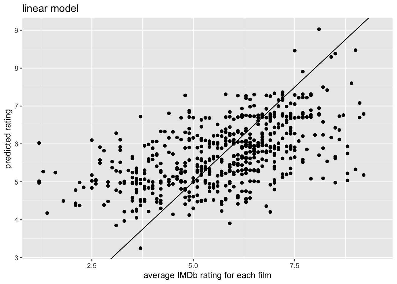
# ℹ 16 more rows

We can use the linear model to predict the rating values for each movie. (Note here that we don’t have test and training data which is definitely a shortcoming in how we’ve modeled!)

movie_wflow_lm |> 
  fit(data = monster_model) |> 
  predict(new_data = monster_model) |> 
  cbind(monster_model) |> 
  ggplot(aes(x = average_rating, y = .pred)) + 
  geom_point() + 
  geom_abline(intercept = 0, slope = 1) + 
  labs(x = "average IMDb rating for each film",
       y = "predicted rating",
       title = "linear model")

Scatterplot describing the relationship between the observed rating and the predicted rating.

movie_wflow_lm |> 
  fit(data = monster_model) |> 
  predict(new_data = monster_model) |> 
  cbind(monster_model) |> 
  select(.pred, average_rating) |> 
  cor(use = "pairwise.complete")

                   .pred average_rating
.pred          1.0000000      0.5382647
average_rating 0.5382647      1.0000000

movie_mod_cart <- decision_tree() |> 
  set_engine(engine = "rpart") |> 
  set_mode(mode = "regression")

movie_wflow_cart <- workflow() |> 
  add_model(movie_mod_cart) |> 
  add_recipe(movie_rec)

movie_wflow_cart |> 
  fit(data = monster_model) |> 
  predict(new_data = monster_model) |> 
  cbind(monster_model) |> 
  ggplot(aes(x = average_rating, y = .pred)) + 
  geom_point() + 
  geom_abline(intercept = 0, slope = 1) +
  labs(x = "average IMDb rating for each film",
       y = "predicted rating",
       title = "regression decision tree")

Scatterplot describing the relationship between the observed rating and the predicted rating. Predicted ratings are given by which terminal node the observation lands. There are 11 terminal nodes, which is why there are 11 possible predicted ratings (note that two of the predicted ratings are very close to each other at roughly 6.2).

movie_wflow_cart |> 
  fit(data = monster_model) |> 
  predict(new_data = monster_model) |> 
  cbind(monster_model) |> 
  select(.pred, average_rating) |> 
  cor(use = "pairwise.complete")

                   .pred average_rating
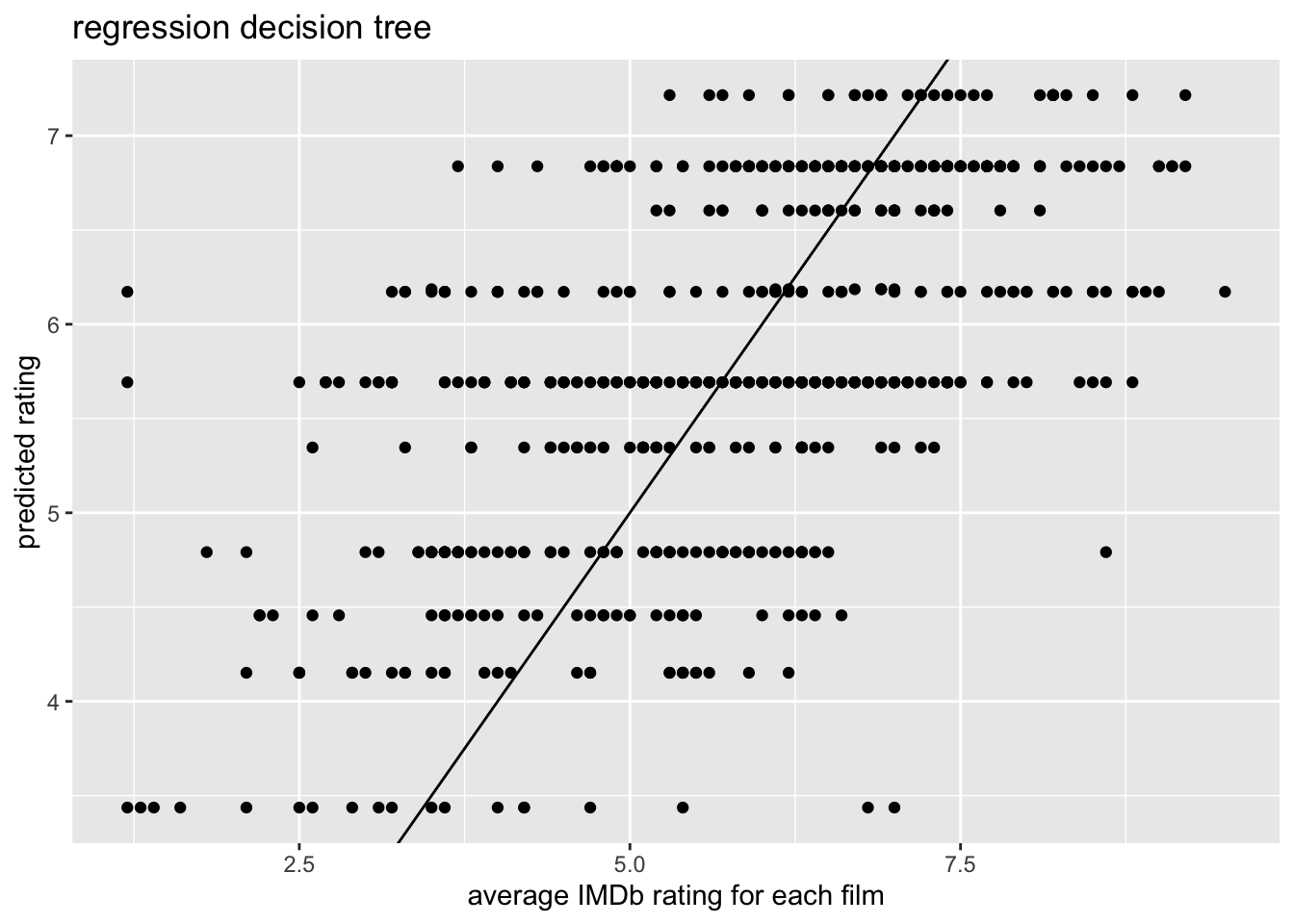
.pred          1.0000000      0.5925846
average_rating 0.5925846      1.0000000

Plotting model

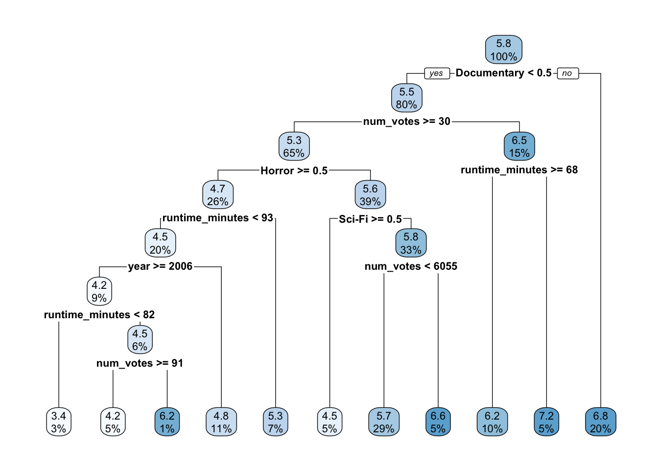
Plotting the decision tree for the regression tree model.

movies_tree <- movie_wflow_cart |> 
  fit(data = monster_model) |> 
  extract_fit_parsnip()

rpart.plot(movies_tree$fit)

A decision tree that shows the different partitions of the explanatory variables. The prediciton is given by the average rating of the films in the terminal node.

praise()

[1] "You are badass!"