Shakespeare Dialogue

library(tidyverse) # ggplot, lubridate, dplyr, stringr, readr...
library(praise)
library(scales)
library(tidytext)
library(devtools)
library(ggwordcloud)
library(png)
library(svglite)

Data

This week we’re exploring dialogue in Shakespeare plays. The dataset this week comes from shakespeare.mit.edu (via github.com/nrennie/shakespeare) which is the Web’s first edition of the Complete Works of William Shakespeare. The site has offered Shakespeare’s plays and poetry to the internet community since 1993.

hamlet <- readr::read_csv('https://raw.githubusercontent.com/rfordatascience/tidytuesday/master/data/2024/2024-09-17/hamlet.csv')
macbeth <- readr::read_csv('https://raw.githubusercontent.com/rfordatascience/tidytuesday/master/data/2024/2024-09-17/macbeth.csv')
romeo_juliet <- readr::read_csv('https://raw.githubusercontent.com/rfordatascience/tidytuesday/master/data/2024/2024-09-17/romeo_juliet.csv')

Romeo & Juliet

After removing stop words, we create wordclouds describing the most common works for both Romeo and Juliet in Romeo & Juliet. Tha anlysis is taken from @deepdk.

romeo_juliet <- romeo_juliet |> 
  filter(character %in% c("Romeo", "Juliet"))

# Create a custom list of words to exclude
custom_stop_words <- data.frame(word = "thou", "thy", "thee", "thine", "art", "hast", "dost", "ere", "o","hath")

word_counts <- romeo_juliet |>
  unnest_tokens(word, dialogue) |>
  anti_join(stop_words) |>  # Remove common stop words
  filter(!str_detect(word, "^[0-9]+$")) |>  # Remove numbers
  anti_join(custom_stop_words) |>  # Remove custom words
  mutate(word = stringr::str_replace(word, "'s", "")) |> 
  count(character, word, sort = TRUE)

word_counts

# A tibble: 1,957 × 3
   character word      n
   <chr>     <chr> <int>
 1 Romeo     love     52
 2 Juliet    romeo    41
 3 Romeo     thy      41
 4 Romeo     thee     38
 5 Juliet    love     35
 6 Juliet    thee     33
 7 Juliet    thy      32
 8 Juliet    night    30
 9 Romeo     death    22
10 Juliet    nurse    20
# ℹ 1,947 more rows

juliet <- word_counts |> 
  filter(character == "Juliet")

romeo <- word_counts |> 
  filter(character == "Romeo")

We wanted to use different fonts, so we load in the MedievalSharp font from Google.

sysfonts::font_add_google("MedievalSharp", "MedievalSharp")
showtext::showtext_auto()

my_font <- "MedievalSharp"

juliet |> 
  #filter(n > 1) |> 
  ggplot(aes(label = word, size = n, color = n)) + 
  #ggwordcloud::geom_text_wordcloud(shape = "cardioid")
  ggwordcloud::geom_text_wordcloud_area(
    mask = png::readPNG("FlipAlphaShakespeare.png"),
    rm_outside = TRUE,
    family = my_font
  ) +
  scale_size_area(max_size = 20) +
  theme_minimal() +
  scale_color_gradient(low = "#03c6fc", high = "#5203fc") + 
  labs(title = "Shakespeare in Words") + 
  theme(
    plot.title = ggtext::element_textbox_simple(
      family = my_font),
    plot.caption = ggtext::element_textbox_simple(
      family = my_font)  )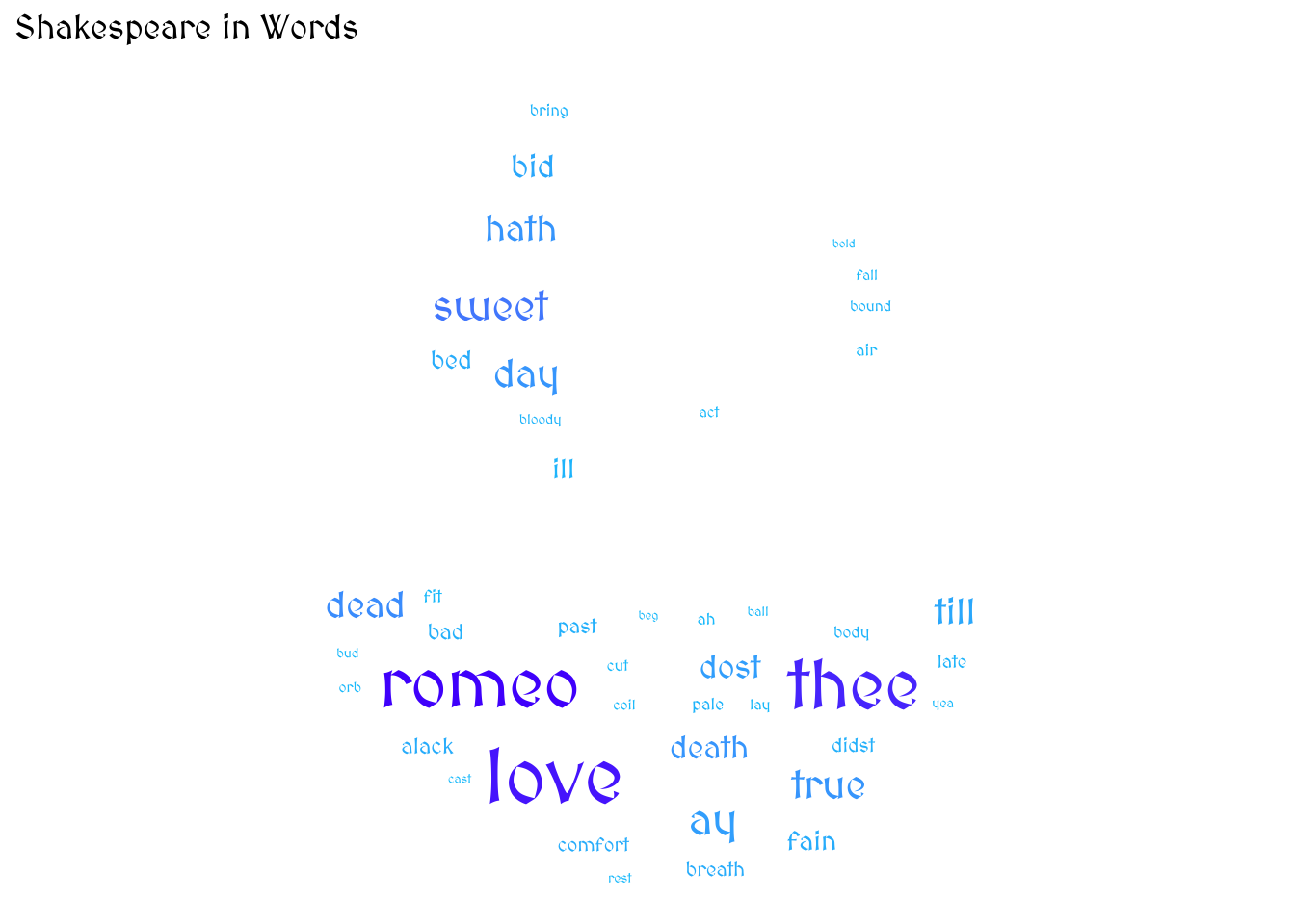

The most common words said by Juliet in Shakespeare’s Romeo & Juliet

romeo |> 
  #filter(n > 1) |> 
  ggplot(aes(label = word, size = n, color = n)) + 
  #ggwordcloud::geom_text_wordcloud(shape = "cardioid")
  ggwordcloud::geom_text_wordcloud_area(
    mask = png::readPNG("AlphaShakespeare.png"),
    rm_outside = TRUE,
    family = my_font
  ) +
  scale_size_area(max_size = 20) +
  theme_minimal() +
  labs(title = "Shakespeare in Words") + 
  theme(
    plot.title = ggtext::element_textbox_simple(
      family = my_font),
    plot.caption = ggtext::element_textbox_simple(
      family = my_font)  ) +
  scale_color_gradient(low = "#a5fc03", high = "#034efc")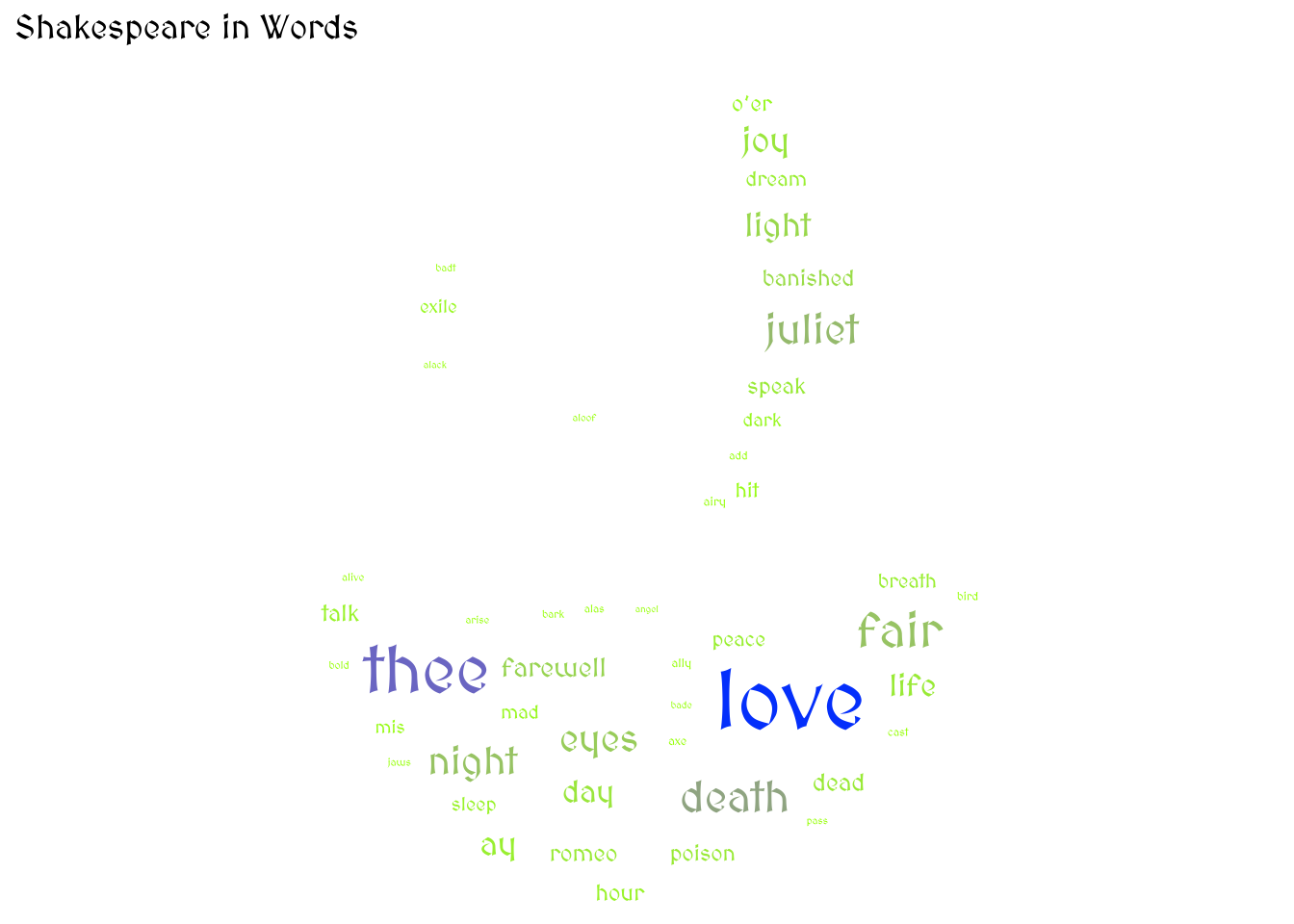

The most common words said by Romeo in Shakespeare’s Romeo & Juliet

praise()

[1] "You are exceptional!"