Rolling Stone Album Rankings

library(tidyverse) # ggplot, lubridate, dplyr, stringr, readr...
library(praise)
library(ggrepel)
library(ggalluvial)

Data

This week we’re looking at album rankings from Rolling Stone. h/t Data is plural. A visual essay from The Pudding looks at what makes an album the greatest of all time, and shares the data they put together for the essay.

rolling_stone <- readr::read_csv('https://raw.githubusercontent.com/rfordatascience/tidytuesday/master/data/2024/2024-05-07/rolling_stone.csv') |>
  mutate(decade = as.factor(floor(release_year/10)*10)) |>
  mutate(top_03 = case_when(
    rank_2003 <= 10 ~ "top 10",
    rank_2003 <= 50 ~ "top 50",
    rank_2003 <= 100 ~ "top 100",
    rank_2003 <= 250 ~ "top 250",
    rank_2003 <= 500 ~ "top 500"),
    
    top_03 = replace_na(top_03, "not top 500"),
    
    top_20 = case_when(
    rank_2020 <= 10 ~ "top 10",
    rank_2020 <= 50 ~ "top 50",
    rank_2020 <= 100 ~ "top 100",
    rank_2020 <= 250 ~ "top 250",
    rank_2020 <= 500 ~ "top 500"),
    
    top_20 = replace_na(top_20, "not top 500")) |>
  mutate(top_03 = factor(top_03, levels = c("top 10", "top 50", "top 100",
                                            "top 250", "top 500", "not top 500")),
         top_20 = factor(top_20, levels = c("top 10", "top 50", "top 100",
                                            "top 250", "top 500", "not top 500")))

rolling_stone |>
  select(artist_gender, decade, top_03, top_20) |>
  group_by(artist_gender, decade, top_03, top_20) |>
  drop_na() |>
  summarize(freq = n()) |>
  data.frame() |>
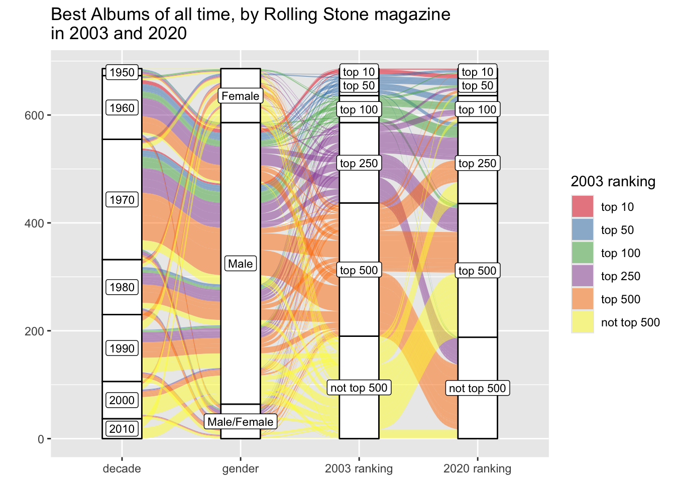
  ggplot(aes(y = freq, axis1 = decade, axis2 = artist_gender, 
                    axis3 = top_03, axis4 = top_20)) +
  geom_alluvium(aes(fill = top_03)) +
  geom_stratum() + 
  geom_label(stat = "stratum", aes(label = after_stat(stratum)), size = 3) +
  scale_x_discrete(limits = c("decade", "gender", "2003 ranking", "2020 ranking")) +
  scale_fill_brewer(palette = "Set1") +
  ggtitle("Best Albums of all time, by Rolling Stone magazine\nin 2003 and 2020") +
  labs(y = "", fill = "2003 ranking")

The alluvial plot is colored by the album rankings in 2003. The connections between the variables show how many albums of each ranking category are in each of the other variable categories. Of particular interest are the connections between the 2003 and 2020 rankings. While there is some commonality across the two ranking time frames, there is also substantial difference. The top ranked albums in 2003 seem to be from male artists, it is difficult to see any changes across gender for 2020 (because the lines have been colored by 2003).

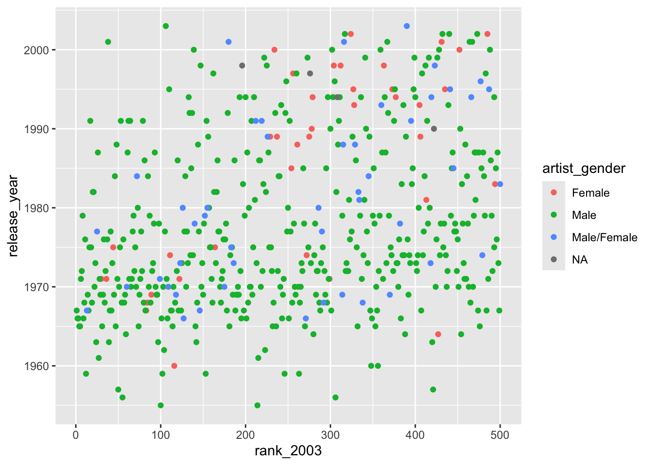
rolling_stone |>
  ggplot(aes(x = rank_2003, y = release_year, color = artist_gender)) + 
  geom_point() + 
  ylim(c(1955, 2003))

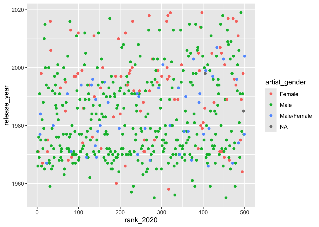
rolling_stone |>
  ggplot(aes(x = rank_2020, y = release_year, color = artist_gender)) + 
  geom_point()

praise()

[1] "You are exquisite!"