Solar Eclipse

library(tidyverse) # ggplot, lubridate, dplyr, stringr, readr...
library(praise)

The Data

This week we’re looking at the paths of solar eclipses in the United States. The data comes from NASA’s Scientific Visualization Studio.

eclipse_annular_2023 <- readr::read_csv('https://raw.githubusercontent.com/rfordatascience/tidytuesday/master/data/2024/2024-04-09/eclipse_annular_2023.csv')
eclipse_total_2024 <- readr::read_csv('https://raw.githubusercontent.com/rfordatascience/tidytuesday/master/data/2024/2024-04-09/eclipse_total_2024.csv')
eclipse_partial_2023 <- readr::read_csv('https://raw.githubusercontent.com/rfordatascience/tidytuesday/master/data/2024/2024-04-09/eclipse_partial_2023.csv')
eclipse_partial_2024 <- readr::read_csv('https://raw.githubusercontent.com/rfordatascience/tidytuesday/master/data/2024/2024-04-09/eclipse_partial_2024.csv')

Putting the 2023 datasets together and the 2024 datasets together so that they can be plotted on the same map. The time variable represents the total duration of the eclipse: the amount of time from when the moon first comes in contact with the sun to when the moon is no longer in contact with the sun.

tot_23 <- eclipse_annular_2023 |>
  mutate(time = eclipse_6 - eclipse_1,
         eclipse = "total") |>
  select(state, name, lat, lon, time, eclipse)

part_23 <- eclipse_partial_2023 |>
  mutate(time = eclipse_5 - eclipse_1,
         eclipse = "partial") |>
  select(state, name, lat, lon, time, eclipse)

eclipse_23 <- rbind(tot_23, part_23) |>
  mutate(time = as.numeric(time))

tot_24 <- eclipse_total_2024 |>
  mutate(time = eclipse_6 - eclipse_1,
         eclipse = "total") |>
  select(state, name, lat, lon, time, eclipse)

part_24 <- eclipse_partial_2024 |>
  mutate(time = eclipse_5 - eclipse_1,
         eclipse = "partial") |>
  select(state, name, lat, lon, time, eclipse)

eclipse_24 <- rbind(tot_24, part_24) |>
  mutate(time = as.numeric(time))

library(ggnewscale)
states <- map_data("state")

ggplot(states) +
  geom_polygon(fill = "white", color = "black", 
               aes(long, lat, group=group)) +
  geom_point(data = filter(eclipse_23, lat < 51 & lat > 24 & lon < 0 & eclipse == "total"), 
             aes(x = lon, y = lat, color = time), size = .1) +
  labs(x = "", y = "") + 
  scale_colour_gradientn(colors = c("blue", "turquoise")) +
  labs(color = "time of overlap (sec)\nannular eclipse") + 
  new_scale_color() + 
  geom_point(data = filter(eclipse_23, lat < 51 & lat > 24 & lon < 0 & eclipse == "partial"), 
             aes(x = lon, y = lat, color = time), size = .001) +
  scale_colour_gradientn(colors = c("red", "pink")) +
  ggtitle("2023 annular solar eclipse") +
  labs(color = "time of overlap (sec)\npartial eclipse")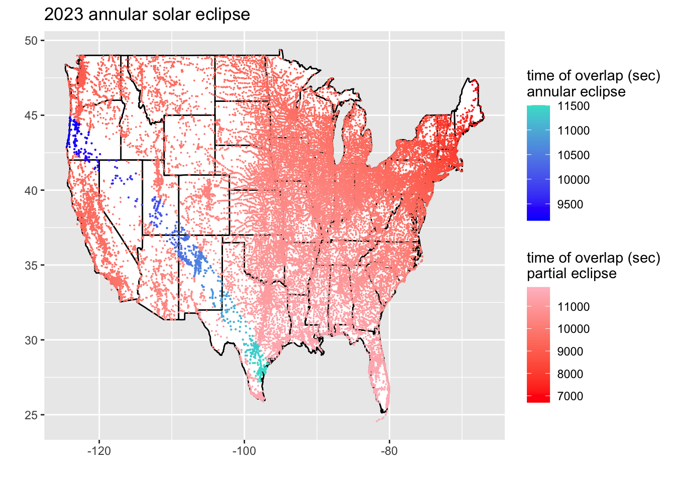

In blue, the path of the 2023 annular solar eclipse. The times represent the difference (in seconds) between when the moon first contacts the sun and when the moon last contacts the sun.

ggplot(states) +
  geom_polygon(fill = "white", color = "black", 
               aes(long, lat, group=group)) +
  geom_point(data = filter(eclipse_24, lat < 51 & lat > 24 & lon < 0 & eclipse == "total"), 
             aes(x = lon, y = lat, color = time), size = .0001) +
  labs(x = "", y = "") + 
  scale_colour_gradientn(colors = c("blue", "turquoise")) +
  labs(color = "time of overlap (sec)\ntotal eclipse") + 
  new_scale_color() + 
  geom_point(data = filter(eclipse_24, lat < 51 & lat > 24 & lon < 0 & eclipse == "partial"), 
             aes(x = lon, y = lat, color = time), size = .0001) +
  scale_colour_gradientn(colors = c("red", "pink")) +
  ggtitle("2024 total solar eclipse") +
  labs(color = "time of overlap (sec)\npartial eclipse")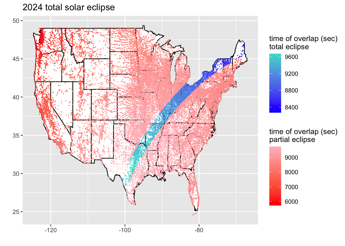

In blue, the path of the 2024 total solar eclipse. The times represent the difference (in seconds) between when the moon first contacts the sun and when the moon last contacts the sun.

praise()

[1] "You are superb!"