X-Men Mutant Moneyball

library(tidyverse) # ggplot, lubridate, dplyr, stringr, readr...
library(praise)

The Data

This week’s data is X-Men Mutant Moneyball from Rally’s Mutant moneyball: a data driven ultimate X-men by Anderson Evans.

While pulling in the data, we use parse_number() to remove all of the $ and % symbols in some of the columns.

mutant_moneyball <- readr::read_csv('https://raw.githubusercontent.com/rfordatascience/tidytuesday/master/data/2024/2024-03-19/mutant_moneyball.csv') |>
  mutate(across(`60s_Appearance_Percent`:PPI90s_oStreet, parse_number))

Wrangling the data

Note that the dataset is currently very wide. And it would be better to have the variables consolidated across decade with a single column referencing the relevant decade for each variable type. We’ll have to pivot_longer() and then wrangle the variable and then pivot_wider() back.

mutant_moneyball

# A tibble: 26 × 45
   Member            TotalIssues TotalIssues60s TotalIssues70s TotalIssues80s
   <chr>                   <dbl>          <dbl>          <dbl>          <dbl>
 1 warrenWorthington         139             61             35             20
 2 hankMcCoy                 119             62             38              9
 3 scottSummers              197             63             69             56
 4 bobbyDrake                123             62             35              6
 5 jeanGrey                  164             63             58             14
 6 alexSummers                68              8             13             43
 7 lornaDane                  48              9             13             19
 8 ororoMunroe               190              0             36            121
 9 kurtWagner                120              0             36             84
10 loganHowlett              167              0             36            115
# ℹ 16 more rows
# ℹ 40 more variables: TotalIssues90s <dbl>, totalIssueCheck <dbl>,
#   TotalValue_heritage <dbl>, TotalValue60s_heritage <dbl>,
#   TotalValue70s_heritage <dbl>, TotalValue80s_heritage <dbl>,
#   TotalValue90s_heritage <dbl>, TotalValue_ebay <dbl>,
#   TotalValue60s_ebay <dbl>, TotalValue70s_ebay <dbl>,
#   TotalValue80s_ebay <dbl>, TotalValue90s_ebay <dbl>, …

The pivot_longer() command below is able to pivot to three name columns, here name1, name2, and name3.

mutant_moneyball |>
  select(-TotalIssues, -totalIssueCheck, 
         -TotalValue_heritage, -TotalValue_ebay) |>
  pivot_longer(cols=-1,
               names_pattern = "(.*)(\\d\\ds)(.*)", 
               names_to = c("name1", "name2", "name3"))

# A tibble: 1,040 × 5
   Member            name1       name2 name3        value
   <chr>             <chr>       <chr> <chr>        <dbl>
 1 warrenWorthington TotalIssues 60s   ""              61
 2 warrenWorthington TotalIssues 70s   ""              35
 3 warrenWorthington TotalIssues 80s   ""              20
 4 warrenWorthington TotalIssues 90s   ""              23
 5 warrenWorthington TotalValue  60s   "_heritage" 929056
 6 warrenWorthington TotalValue  70s   "_heritage" 154585
 7 warrenWorthington TotalValue  80s   "_heritage"  23957
 8 warrenWorthington TotalValue  90s   "_heritage"    960
 9 warrenWorthington TotalValue  60s   "_ebay"      23335
10 warrenWorthington TotalValue  70s   "_ebay"       3362
# ℹ 1,030 more rows

But the name of the value should be name1 and name3 pasted together.

mutant_moneyball |>
  select(-TotalIssues, -totalIssueCheck, 
         -TotalValue_heritage, -TotalValue_ebay) |>
  pivot_longer(cols=-1,
               names_pattern = "(.*)(\\d\\ds)(.*)", 
               names_to = c("name1", "name2", "name3")) |>
  mutate(variable = paste(name1, name3, sep = "")) 

# A tibble: 1,040 × 6
   Member            name1       name2 name3        value variable           
   <chr>             <chr>       <chr> <chr>        <dbl> <chr>              
 1 warrenWorthington TotalIssues 60s   ""              61 TotalIssues        
 2 warrenWorthington TotalIssues 70s   ""              35 TotalIssues        
 3 warrenWorthington TotalIssues 80s   ""              20 TotalIssues        
 4 warrenWorthington TotalIssues 90s   ""              23 TotalIssues        
 5 warrenWorthington TotalValue  60s   "_heritage" 929056 TotalValue_heritage
 6 warrenWorthington TotalValue  70s   "_heritage" 154585 TotalValue_heritage
 7 warrenWorthington TotalValue  80s   "_heritage"  23957 TotalValue_heritage
 8 warrenWorthington TotalValue  90s   "_heritage"    960 TotalValue_heritage
 9 warrenWorthington TotalValue  60s   "_ebay"      23335 TotalValue_ebay    
10 warrenWorthington TotalValue  70s   "_ebay"       3362 TotalValue_ebay    
# ℹ 1,030 more rows

Then we need to pivot_wider() so that the columns of interest are separated.

mutant_moneyball_clean <- mutant_moneyball |>
  select(-TotalIssues, -totalIssueCheck, 
         -TotalValue_heritage, -TotalValue_ebay) |>
  pivot_longer(cols=-1,
               names_pattern = "(.*)(\\d\\ds)(.*)", 
               names_to = c("name1", "name2", "name3")) |>
  mutate(variable = paste(name1, name3, sep = "")) |>
  select(Member, decade = name2, value, variable) |>
  pivot_wider(names_from = variable, values_from = value)

mutant_moneyball_clean

# A tibble: 104 × 12
   Member            decade TotalIssues TotalValue_heritage TotalValue_ebay
   <chr>             <chr>        <dbl>               <dbl>           <dbl>
 1 warrenWorthington 60s             61              929056           23335
 2 warrenWorthington 70s             35              154585            3362
 3 warrenWorthington 80s             20               23957             583
 4 warrenWorthington 90s             23                 960              97
 5 hankMcCoy         60s             62              929776           23377
 6 hankMcCoy         70s             38               20705            1224
 7 hankMcCoy         80s              9                6631             289
 8 hankMcCoy         90s             10                 881              82
 9 scottSummers      60s             63              933616           23420
10 scottSummers      70s             69              188635            5431
# ℹ 94 more rows
# ℹ 7 more variables: `_Appearance_Percent` <dbl>, PPI_heritage <dbl>,
#   PPI_ebay <dbl>, TotalValue_wiz <dbl>, TotalValue_oStreet <dbl>,
#   PPI_wiz <dbl>, PPI_oStreet <dbl>

The data is now in a format that will make graphing easy!

Graphing

Comparing different valuations

mutant_moneyball_clean |>
  #ggplot(aes(x = PPI_wiz, y = PPI_ebay)) + 
  ggplot(aes(x = PPI_wiz, y = PPI_oStreet)) + 
  geom_point(aes(size = TotalIssues, color = Member)) +
  geom_abline(intercept = 0, slope = 1) + 
  ggrepel::geom_label_repel(aes(label = Member), max.overlaps = 15,
                            size = 2) +
  facet_wrap(~decade, scales = "free") + 
  theme(legend.position = "none") +
  labs(x = "Price per issue, Wizard Price Guide",
       y = "Price per issues, Overstreet Price Guide",
       title = "Price and frequency for X-Men commic books\nincluding each of the given characters",
       subtitle = "Size of dot proportional to the number of issues character appeared in")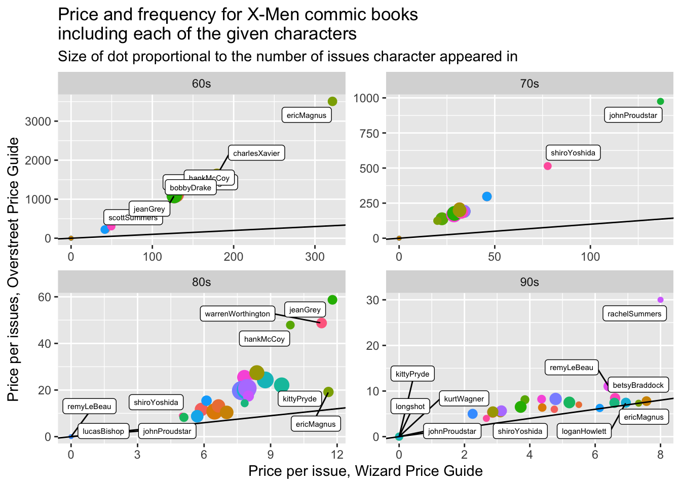

Difference in price per issue for two different price guides: Wizard and Overstreet. Note that the Overstreet Price Guide consistently estimates the issues as higher priced than the Wizard Price Guide.

praise()

[1] "You are astonishing!"