People and events on Leap Days

Author

Jo Hardin

Published

February 27, 2024

library(tidyverse) # ggplot, lubridate, dplyr, stringr, readr...
library(babynames)
library(praise)

The Data

Happy Leap Day! This week’s data comes from the February 29 article on Wikipedia.

February 29 is a leap day (or “leap year day”), an intercalary date added periodically to create leap years in the Julian and Gregorian calendars.

One event that’s missing from Wikipedia’s list: R version 1.0 was released on February 29, 2000.

events <- readr::read_csv('https://raw.githubusercontent.com/rfordatascience/tidytuesday/master/data/2024/2024-02-27/events.csv')
births <- readr::read_csv('https://raw.githubusercontent.com/rfordatascience/tidytuesday/master/data/2024/2024-02-27/births.csv')
deaths <- readr::read_csv('https://raw.githubusercontent.com/rfordatascience/tidytuesday/master/data/2024/2024-02-27/deaths.csv')

babynames |>
  filter(name == "Matthew" | name == "John" | name == "Federica" | name == "Johanna" | name == "Clara") |>
  filter(sex == "F") |>
  ggplot(aes(x = year, y = n, color = name)) +
  geom_line(aes(lty = sex))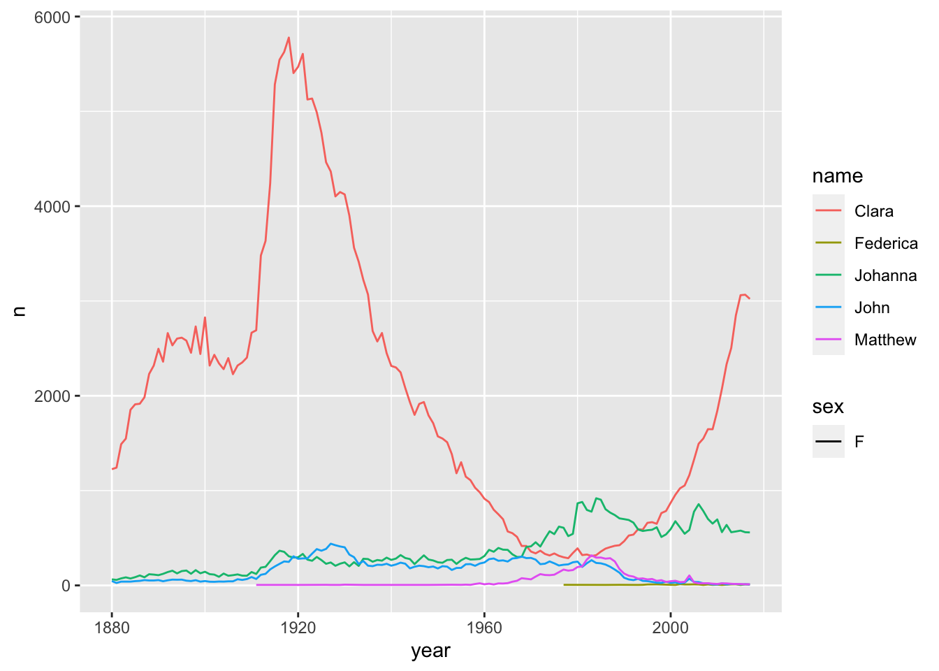

babynames |> filter(name == "Jaguar")

# A tibble: 8 × 5
   year sex   name       n       prop
  <dbl> <chr> <chr>  <int>      <dbl>
1  1992 M     Jaguar     8 0.00000381
2  1994 M     Jaguar     8 0.00000393
3  1995 M     Jaguar    12 0.00000597
4  2002 M     Jaguar     7 0.00000339
5  2004 M     Jaguar     5 0.00000237
6  2013 M     Jaguar     6 0.00000298
7  2014 M     Jaguar     5 0.00000245
8  2017 M     Jaguar     6 0.00000306

births <- births |>
  separate(person, c("Fname", "Lname", "other"))

leap_names <- births |>  # create a list of duplicate leap names
  group_by(Fname) |>
  summarize(count = n()) |>
  filter(count >= 2) 

leap_names

# A tibble: 7 × 2
  Fname   count
  <chr>   <int>
1 Antonio     2
2 Dave        2
3 Frank       2
4 James       3
5 Lena        2
6 Pedro       2
7 Richard     2

leap_births <- babynames |>
  filter(name %in% leap_names$Fname) |> # names that happen at least twice 
  group_by(name, year) |>
  mutate(diff = n - lag(n),             # measures women minus men (only for M rows)
         diff_plus = n - lead(n)) |>    # measures men minus women (only for F rows)
  mutate(keep_sex = case_when(
    n > abs(diff) ~ "M", 
    n > abs(diff_plus) ~ "F",
    n < abs(diff) ~ "F",
    n < abs(diff_plus) ~ "M",
    TRUE ~ sex
  )) |>
  filter(sex == keep_sex) 
  
leap_births

# A tibble: 966 × 8
# Groups:   name, year [966]
    year sex   name        n     prop  diff diff_plus keep_sex
   <dbl> <chr> <chr>   <int>    <dbl> <int>     <int> <chr>   
 1  1880 F     Lena      603 0.00618     NA        NA F       
 2  1880 M     James    5927 0.0501    5905        NA M       
 3  1880 M     Frank    3242 0.0274    3229        NA M       
 4  1880 M     Richard   728 0.00615     NA        NA M       
 5  1880 M     Dave      131 0.00111     NA        NA M       
 6  1880 M     Pedro      31 0.000262    NA        NA M       
 7  1880 M     Antonio    26 0.000220    NA        NA M       
 8  1881 F     Lena      555 0.00561     NA        NA F       
 9  1881 M     James    5441 0.0502    5417        NA M       
10  1881 M     Frank    2834 0.0262    2825        NA M       
# ℹ 956 more rows

pal <- c("#004949","#009292","#ff6db6",
 "#490092","#006ddb","#b66dff","#6db6ff",
 "#920000","#24ff24","#ffff6d")

leap_births |>
  ggplot(aes(x = year, y = n)) + 
  geom_line(aes(color = name, lty = sex)) +
  geom_point(data = filter(births, Fname %in% leap_names$Fname),
             aes(color = Fname, x = year_birth), y = 75000, size = 3) +
  xlim(1880, 2020) +
  scale_linetype_manual(values = c("dashed", "solid")) + 
  scale_color_manual(values = pal) +
  labs(y = "",
       x = "",
       title = "Number of births with given name at each year",
       subtitle = "Dots indicate a leap day baby famous person")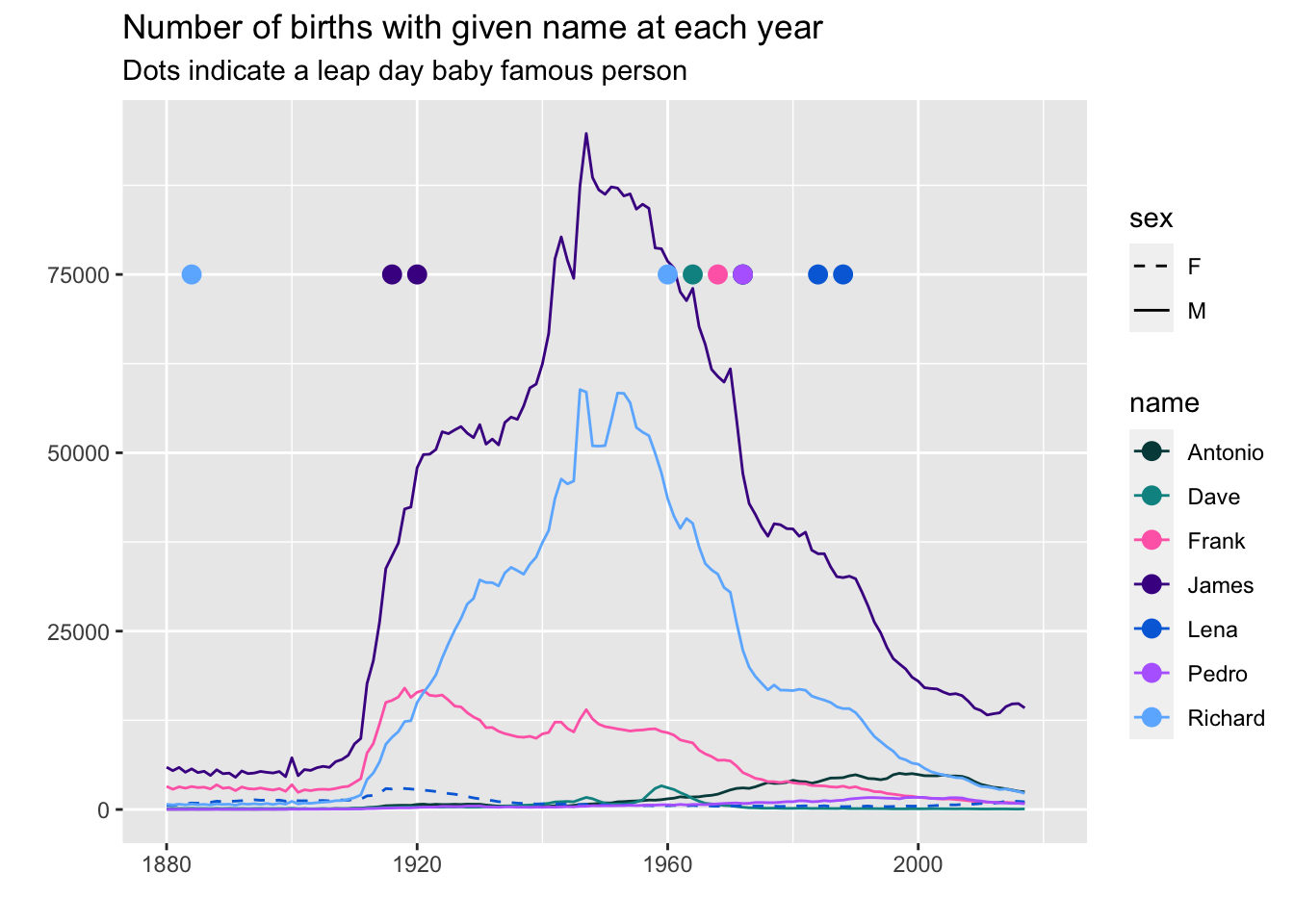

Line plots showing the trends of baby naming in the US from 1880 to 2017. The seven people were chosen because their first names showed up at least twice in the list of leap day people. Across the board, the names were most popular from about 1940 to 1970. — Trends in the US for babynames for “famous” people who were born on leap day. The seven people were chosen because their first names showed up at least twice in the list of leap day people.

leap_births2 <- babynames |>
  filter(name %in% births$Fname) |> # all the names in the leap year data 
  group_by(name, year) |>
  mutate(diff = n - lag(n),             # measures women minus men (only for M rows)
         diff_plus = n - lead(n)) |>    # measures men minus women (only for F rows)
  mutate(keep_sex = case_when(
    n > abs(diff) ~ "M", 
    n > abs(diff_plus) ~ "F",
    n < abs(diff) ~ "F",
    n < abs(diff_plus) ~ "M",
    TRUE ~ sex
  )) |>
  filter(sex == keep_sex) |>
  ungroup() |>
  group_by(name) |>
  mutate(tot_names = sum(n)) |>
  filter(tot_names > 1000000)
  
leap_births2 |>
  slice_head(n=1) |>
  arrange(tot_names)

# A tibble: 10 × 9
# Groups:   name [10]
    year sex   name         n      prop  diff diff_plus keep_sex tot_names
   <dbl> <chr> <chr>    <int>     <dbl> <int>     <int> <chr>        <int>
 1  1880 F     Jessica      7 0.0000717    NA        NA F          1044939
 2  1880 M     Edward    2364 0.0200       NA        NA M          1288725
 3  1880 M     Mark        85 0.000718     NA        NA M          1349865
 4  1884 F     Patricia     6 0.0000436    NA        NA F          1571692
 5  1880 M     Richard    728 0.00615      NA        NA M          2563082
 6  1880 M     David      869 0.00734      NA        NA M          3611329
 7  1880 M     William   9532 0.0805     9502        NA M          4102604
 8  1880 M     Michael    354 0.00299      NA        NA M          4350824
 9  1880 M     John      9655 0.0815     9609        NA M          5115466
10  1880 M     James     5927 0.0501     5905        NA M          5150472

leap_births2 |>
  ggplot(aes(x = year, y = n)) + 
  geom_line(aes(color = name, lty = sex)) +
  geom_point(data = filter(births, Fname %in% leap_births2$name),
             aes(color = Fname, x = year_birth), y = 75000, size = 3) +
  xlim(1880, 2020) +
  scale_linetype_manual(values = c("dashed", "solid")) + 
  scale_color_manual(values = pal) +
  labs(y = "",
       x = "",
       title = "Number of births with given name at each year",
       subtitle = "Dots indicate a leap day baby famous person")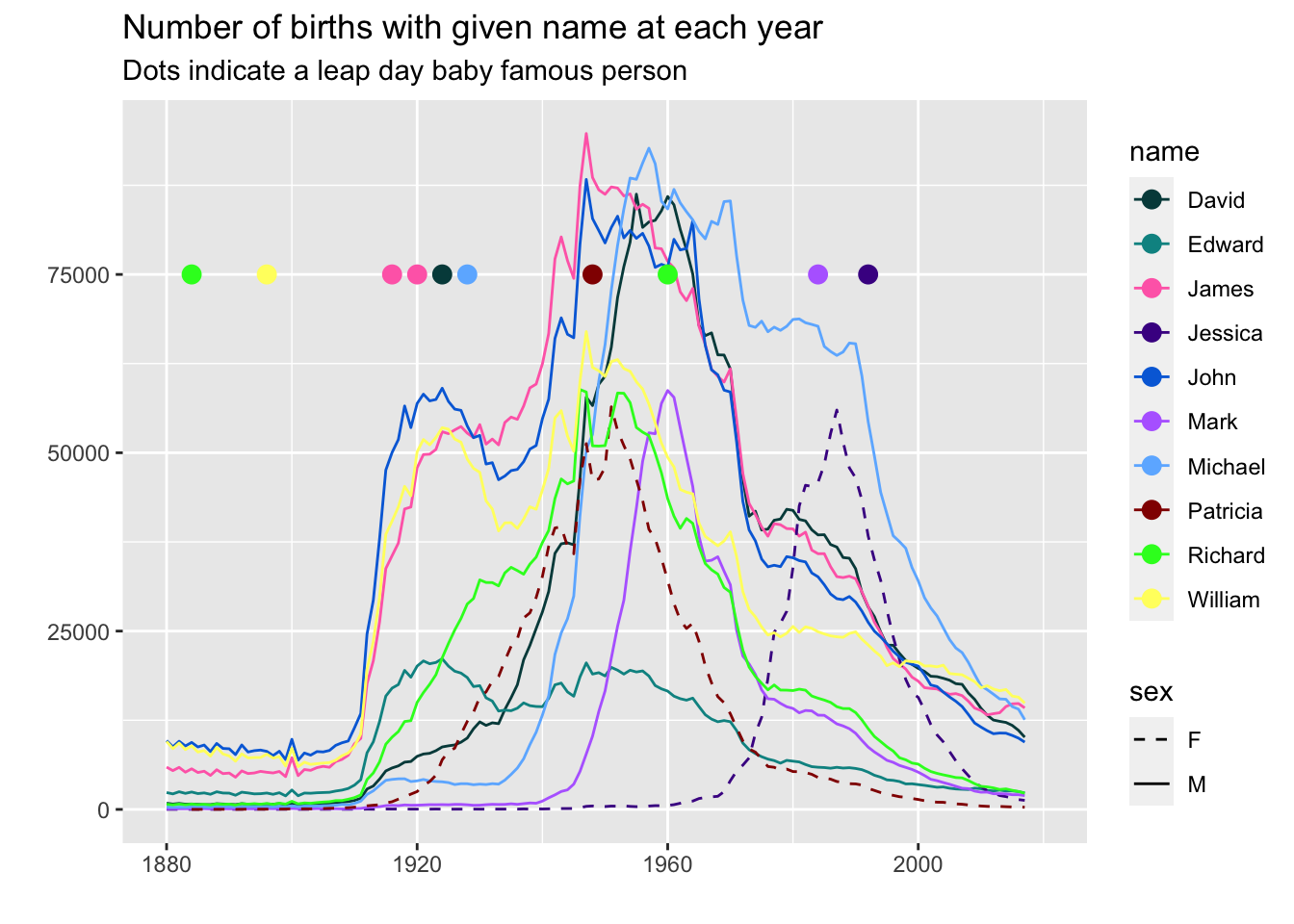

Line plots showing the trends of baby naming in the US from 1880 to 2017. The names were chosen because, of the leap day birthday set, they were the names that were the most popular in the US across time. Across the board, the names were most popular from about 1940 to 1970. — Trends in the US for babynames for “famous” people who were born on leap day. The ten people were chosen because, of the leap day birthday set, they were the names that were most popular in the US across time.

praise()

[1] "You are cat's pajamas!"