Groundhog Dog

library(tidyverse) # ggplot, lubridate, dplyr, stringr, readr...
library(praise)

The Data

On February 2nd of each year, the groundhog comes out of their hole. If the groundhog sees its own shadow, it fortells six more weeks of winter weather. Today’s data include Groundhog Day Predictions from groundhog-day.com. If you haven’t seen it, you should check out the fantastic 1993 movie, Groundhog Day.

groundhogs <- readr::read_csv('https://raw.githubusercontent.com/rfordatascience/tidytuesday/master/data/2024/2024-01-30/groundhogs.csv')
predictions <- readr::read_csv('https://raw.githubusercontent.com/rfordatascience/tidytuesday/master/data/2024/2024-01-30/predictions.csv')

Plotting the data

Punxsutawney Phil is arguably the most famous groundhog of those who make annual predictions. He is listed as groundhog number 1. The id values are sequentially ordered by those groundhogs (really cities / communities) with the most annual predictions.

predictions |>
  filter(id <= 6) |> 
  filter(year > 1900) |>
  drop_na(shadow) |>
  ggplot(aes(x = year, y = shadow, color = as.factor(id))) +
  geom_jitter(width = 0, height = 0.1) +
  facet_wrap(~id) +
  labs(x = "", y = "", title = "Did the groundhog see its shadow?",
       color = "groundhog ID")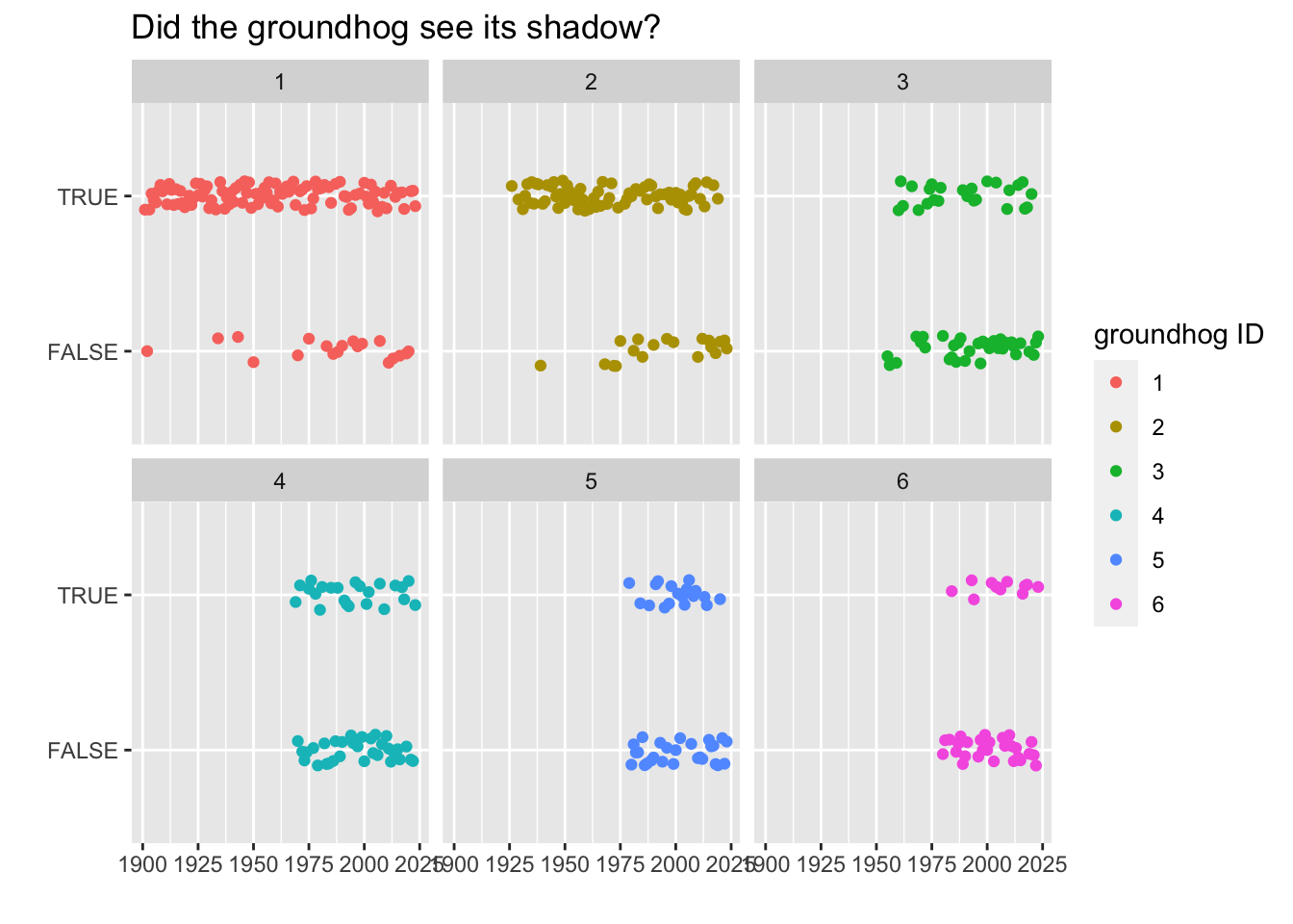

For the six groundhogs with the most predictions, over time, whether they saw their shadow or not.

predictions |>
  #filter(id <=10) |>
  drop_na(shadow) |>
  group_by(id) |>
  summarize(prop_true = mean(shadow),
            num_pred = n()) |>
  ggplot(aes(x = id, y = prop_true)) +
  geom_point(aes(size = num_pred)) +
  labs(x = "groundhog ID", y = "", title = "Proportion of times the groundhog saw its shadow",
       size = "number of predictions")

Each dot represents a separate groundhog. The larger dots are those groundhogs who have made many predictions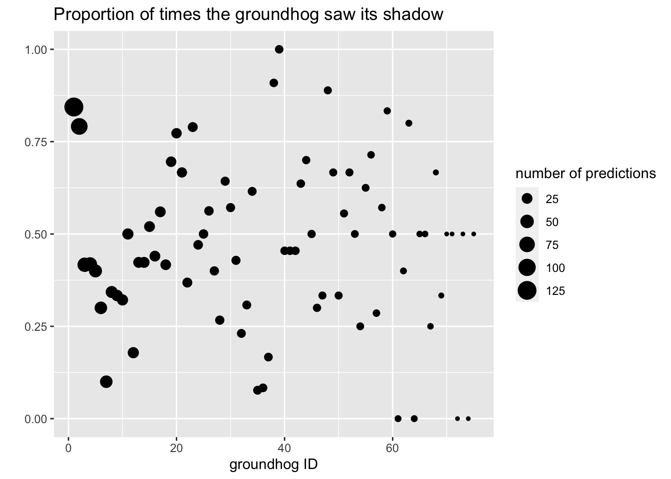. There does not seems to be any relationship between the number of predictions and the proportion of times the groundhog saw its shadow.

The type of groundhog is an interesting variable. Although most of the groundhogs are actual groundhogs, some of them are a different type of animal (opossum, prairie dog, cat, beaver,…) and some are pretty random (taxidermied groundhog, person in a groundhog suit, animatronic groundhog, …). We create a new variable to bin the type into three categories of: groundhog, type of groundhog (but not a real groundhog), or not a groundhog.

location_pred <- predictions |>
  drop_na(shadow) |>
  group_by(id) |>
  summarize(prop_true = mean(shadow),
            num_pred = n()) |>
  mutate(half_pred = ifelse(prop_true >= 0.5, TRUE, FALSE)) |>
  full_join(groundhogs, by = "id") |>
  mutate(groundhog = case_when(
    type == "Groundhog" ~ "groundhog",
    grepl("groundhog", type, ignore.case = TRUE) ~ "type of groundhog",
    TRUE ~ "not a groundhog")) 

states <- map_data("state")

ggplot(states) +
  geom_polygon(fill = "white", colour = "black", 
               aes(long, lat, group=group)) +
  geom_point(data = location_pred, 
             aes(x = longitude, y = latitude, color = groundhog, size = num_pred)) +
  labs(x = "", y = "", size = "number of predictions", color = "")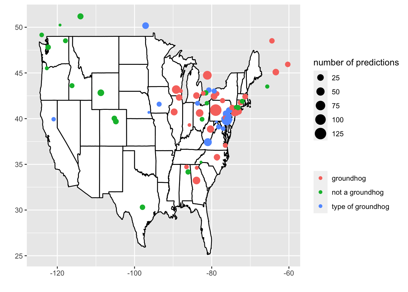

Using longitude and latitude, each of the groundhog locations is plotted on a US map. Some of the points fall off the map because they are in Canada. The points are sized by the number of predictions and colored by the type of groundhog.

praise()

[1] "You are slick!"