US House Results

library(tidyverse) # ggplot, lubridate, dplyr, stringr, readr...
library(tidytext)
library(praise)
library(paletteer)
library(geofacet)
library(usmap)
library(gganimate)
library(transformr)

The Data

The data this week comes from the MIT Election Data and Science Lab (MEDSL).

house <- read_csv("house.csv") |>
  mutate(party_new = case_when(
    party == "DEMOCRAT" ~ "democrat",
    party == "REPUBLICAN" ~ "republican",
    party == "LIBERTARIAN" ~ "libertarian",
    party == "INDEPENDENT" ~ "independent",
    party == "CONSERVATIVE" ~ "conservative",
    party == "GREEN" ~ "green",
    TRUE ~ "other"
  ))

house |>
  group_by(party) |>
  summarize(count_party = n()) |>
  arrange(desc(count_party))

# A tibble: 478 × 2
   party            count_party
   <chr>                  <int>
 1 DEMOCRAT                9908
 2 REPUBLICAN              9705
 3 <NA>                    3858
 4 LIBERTARIAN             2769
 5 INDEPENDENT             1217
 6 CONSERVATIVE             668
 7 GREEN                    513
 8 NATURAL LAW              371
 9 WORKING FAMILIES         283
10 LIBERAL                  266
# ℹ 468 more rows

house |>
  group_by(party_new) |>
  summarize(count_party = n()) |>
  arrange(desc(count_party))

# A tibble: 7 × 2
  party_new    count_party
  <chr>              <int>
1 democrat            9908
2 republican          9705
3 other               7672
4 libertarian         2769
5 independent         1217
6 conservative         668
7 green                513

Some maps

house |>
  filter(year == 2022) |>
  filter(party_new %in% c("democrat", "republican")) |>
  group_by(state_po, party_new) |>
  summarize(vote_count = sum(candidatevotes)) |>
  ggplot(aes(y = vote_count, x = party_new, fill = party_new)) +
  geom_bar(stat = "identity") + 
  coord_flip() + 
  theme(axis.text.x = element_text(angle = 45, vjust = 0.5, hjust=1)) +
  facet_geo(~state_po, grid = "us_state_grid2")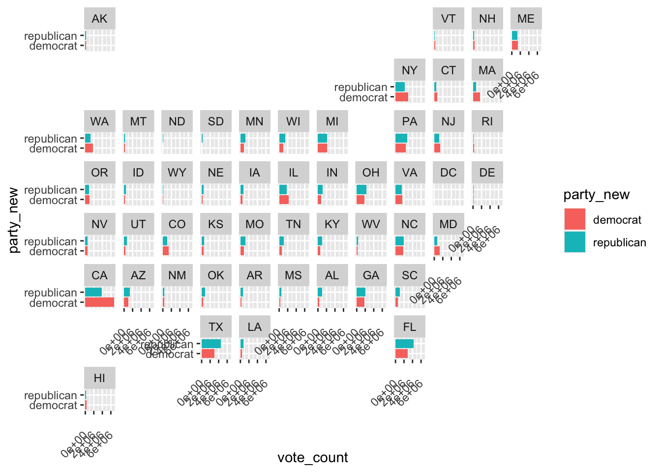

Alas, OF COURSE, districts are different from counties. There are way more counties than districts. So the vast majority of counties are not colored in.

house_county <- house |>
  mutate(fips = case_when(
    state_fips < 10 ~ paste0("0",state_fips,district, sep = ""),
    TRUE ~ paste(state_fips,district,sep="")
  )) |>
  filter(party_new %in% c("democrat", "republican")) |>
  group_by(state, district, year) |>
  mutate(proportions = candidatevotes / sum(candidatevotes)) |>
  select(state_fips, district, fips, proportions) |>
  filter(year == 2016) 

usmap::plot_usmap(regions = "counties", 
                  data = house_county, 
                  values = "proportions",
                  linewidth = 0) + 
  scale_fill_continuous(type = "viridis", 
                        name = "Purpleness")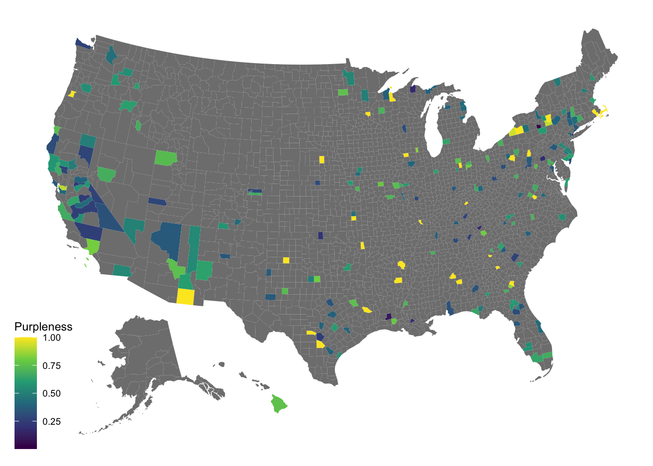

So instead, let’s look at the state map. Here the total number of votes cast is summed up over all of the districts in a particular state.

house_state <- house |>
  filter(party_new %in% c("democrat", "republican")) |>
  group_by(state, year, party_new) |>
  summarize(party_count = sum(candidatevotes)) |>
  summarize(proportions = party_count / sum(party_count), party_new = party_new) |>
  mutate(year = as.integer(year))

p <- usmap::plot_usmap(regions = "state", 
                  data = house_state, 
                  values = "proportions",
                  linewidth = 0) + 
  scale_fill_gradient(low = "red", high = "darkblue",
                        name = "Purpleness") + 
  transition_time(year) +
  labs(subtitle = "Year: {frame_time}",
       title = "Out of total votes cast for Republicans and Democrats, the proportion\n that went to democrats.",
       caption = "Data credit: @MIT Election Data and Science Lab")

animate(p)

Choropleth map of the united states colored by the proportion of votes that went to a Democrat.

praise()

[1] "You are best!"