Haunted Places

library(tidyverse) # ggplot, lubridate, dplyr, stringr, readr...
library(tidytext)
library(praise)
library(sf)
library(paletteer)

The Data

This week’s data is a compilation of Haunted Places in the United States. The dataset was compiled by Tim Renner, using The Shadowlands Haunted Places Index, and shared on data.world.

haunted_places <- read_csv("haunted_places.csv") %>%
  mutate(index = seq(1:n()))

haunted_places |>
  filter(state == "Ohio") |>
  arrange(desc(longitude))

# A tibble: 477 × 11
   city       country description location state state_abbrev longitude latitude
   <chr>      <chr>   <chr>       <chr>    <chr> <chr>            <dbl>    <dbl>
 1 Medina     United… "Formerly … Light &… Ohio  OH               139.     -34.4
 2 Nelsonvil… United… "It was st… Old Mou… Ohio  OH               -79.0     43.2
 3 New Middl… United… "Old summe… Locust … Ohio  OH               -80.5     40.9
 4 New Middl… United… "A young m… State R… Ohio  OH               -80.6     41.0
 5 New Water… United… "A little … Hisey R… Ohio  OH               -80.6     40.9
 6 Calcutta   United… "Beaver Cr… East Li… Ohio  OH               -80.6     40.7
 7 Calcutta   United… "Beaver Cr… East Li… Ohio  OH               -80.6     40.7
 8 Calcutta   United… "Gretchen’… East Li… Ohio  OH               -80.6     40.7
 9 Columbian… United… "the bridg… Little … Ohio  OH               -80.6     40.7
10 East Live… United… "Part of a… Beaver … Ohio  OH               -80.6     40.7
# ℹ 467 more rows
# ℹ 3 more variables: city_longitude <dbl>, city_latitude <dbl>, index <int>

usa <- sf::st_as_sf(maps::map("state", fill = TRUE, plot = FALSE))

haunted_map <- haunted_places |>
  filter(city_longitude > -130) |>
  mutate(location = str_to_lower(location)) |>
  mutate(place = case_when(
    grepl("school", location) ~ "school",
    grepl("university", location) ~ "school",
    grepl("college", location) ~ "school",
    grepl("inn",  location) ~ "hotel",
    grepl("hotel",  location) ~ "hotel",
    grepl("motel",  location) ~ "hotel",
    grepl("cemetery",  location) ~ "cemetery",
    grepl("hospital",  location) ~ "hospital",
    grepl("house",  location) ~ "house",
    grepl("bridge",  location) ~ "bridge",
    grepl("park",  location) ~ "park",
    TRUE ~ "other"))

ggplot(usa) +
  geom_sf(color = "black", fill = "white", size = 1) +
  geom_point(data = haunted_map, 
             aes(y = city_latitude, x = city_longitude, color = place), 
             size= .2) +
  scale_color_paletteer_d("RColorBrewer::Dark2") + 
  #ggthemes::scale_color_colorblind() +
  labs(x = "", y = "",
       title = "Haunted places across the US")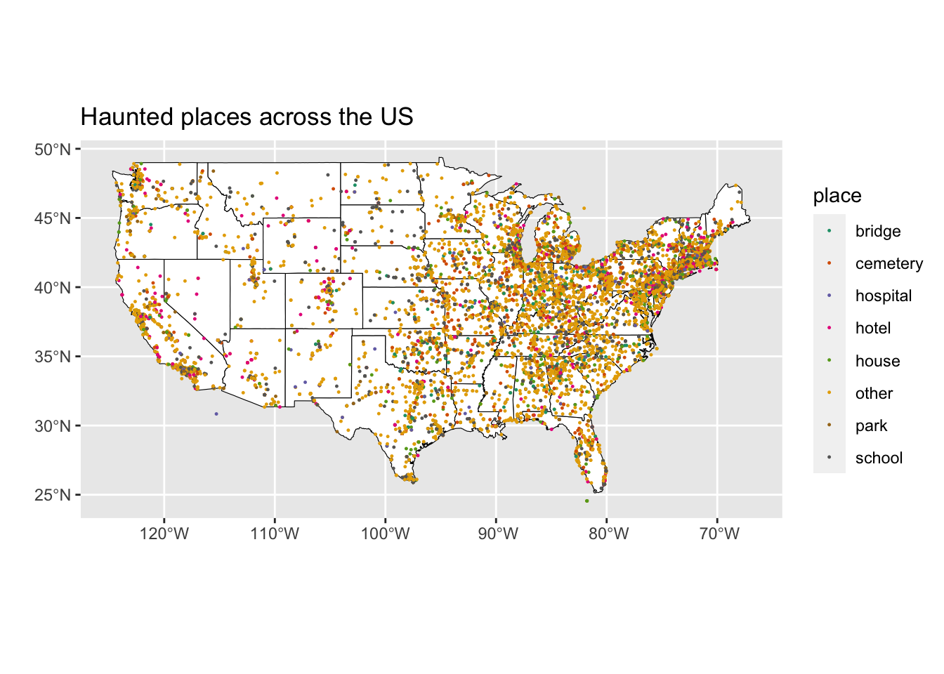

haunted_loc <- haunted_places |>
  unnest_tokens(word_location, location)

haunted_loc |>
  select(word_location) |>
  group_by(word_location) |>
  summarize(word_count = n()) |>
  arrange(desc(word_count)) |>
  head(n = 20)

# A tibble: 20 × 2
   word_location word_count
   <chr>              <int>
 1 school              1217
 2 the                  989
 3 cemetery             751
 4 high                 700
 5 old                  599
 6 house                502
 7 university           500
 8 road                 437
 9 of                   406
10 college              373
11 park                 354
12 state                307
13 inn                  279
14 hotel                272
15 st                   253
16 bridge               252
17 and                  227
18 hospital             222
19 hill                 208
20 middle               203

places <- c("school", "cemetery", "house", "university", "college", "park", "inn", "hotel", "bridge", "hospital")

haunted_loc |>
  filter(word_location %in% places) |>
  group_by(index) |>
  distinct(word_location) |>
  summarize(num_places = n()) |>
  arrange(desc(num_places)) |>
  head(n = 20)

# A tibble: 20 × 2
   index num_places
   <int>      <int>
 1  4655          3
 2  9774          3
 3    40          2
 4   125          2
 5   141          2
 6   159          2
 7   173          2
 8   231          2
 9   452          2
10   459          2
11   651          2
12   705          2
13   714          2
14   999          2
15  1179          2
16  1258          2
17  1352          2
18  1384          2
19  1519          2
20  1635          2