Time Zones

library(tidyverse)
library(tidytext)
library(praise)
library(scales)

The Data

The data this week comes from the IANA tz database via the {clock} and {tzdb} packages. Special thanks to Davis Vaughan for the assist in preparing this data!

timezones <- read_csv("timezones.csv")
transitions <- read_csv("transitions.csv")
timezone_countries <- read_csv("timezone_countries.csv")
countries <- read_csv("countries.csv")

Making a Time Zone plot

The code is taken almost directly from @mvbloois.

library(tidyverse) 
library(patchwork) 
library(sf) 
library(showtext) 
font_add_google("Oswald", "font") 
showtext_auto() 
showtext_opts(dpi = 300) 

world_map <- map_data("world") 
pal <- c("#E40303", "#FF8C00", "#FFED00", "#008026", "#24408E", "#732982") 
now <- Sys.time() 
data <- transitions %>% 
  group_by(zone) %>% 
  filter(lubridate::as_datetime(begin) < now) %>% 
  filter(begin == max(begin)) %>% 
  ungroup() %>% 
  inner_join( timezones, by = "zone" ) %>% 
  mutate(offset_hr = offset / 3600) 

plt_1 <- ggplot() + 
  geom_map(data = world_map, 
           map = world_map, aes(map_id = region), fill = "lightblue") + 
  geom_point(data = data, 
             aes(x = longitude, y = latitude, 
                 colour = factor(offset_hr)), show.legend = FALSE) + 
  scale_colour_manual(values = rep(pal, times = 6)) + 
  coord_equal() + 
  labs(title = "What time is it?", 
       subtitle = "Offset from UTC for various cities in the world on Tuesday March 28, 2023") + 
  theme_void() + 
  theme( plot.title = element_text(family = "font", hjust = 0.5, size = 32), 
         plot.subtitle = element_text(family = "font", hjust = 0.5) ) 

levels <- c("+13","+13¾","+14","-11","-10","-9½","-9","-8","-7","-6","-5","-4","-3","-2½","-2","-1","0","+1", "+2","+3","+4","+4½","+5","+5½","+5¾","+6","+6½","+7","+8","+8¾","+9","+9½","+10","+10½","+11","+12") 

offsets <- data %>% 
  distinct(offset_hr) %>% 
  mutate(offset_txt = scales::label_number(style_positive = "plus")(offset_hr), offset_txt = str_remove(offset_txt, ".00"), 
         offset_txt = str_replace(offset_txt, ".50", "½"), 
         offset_txt = str_replace(offset_txt, ".75", "¾")) %>% 
  mutate(offset_txt = factor(offset_txt, levels = levels)) 

plt_2 <- offsets %>% 
  ggplot() + 
  geom_tile(aes(x = offset_txt, y = 1, fill = factor(offset_hr)), 
            show.legend = FALSE) + 
  geom_text(aes(x = offset_txt, y = 1, label = factor(offset_txt)), 
            family = "font", colour = "white", size = 2.5) + 
  scale_fill_manual(values = rep(pal, times = 6)) + 
  labs(caption = "Data: IANA tz database\nCode: @mvbloois") + 
  coord_equal() + 
  theme_void() + 
  theme( plot.caption = element_text(family = "font") ) 

plt_1 / plt_2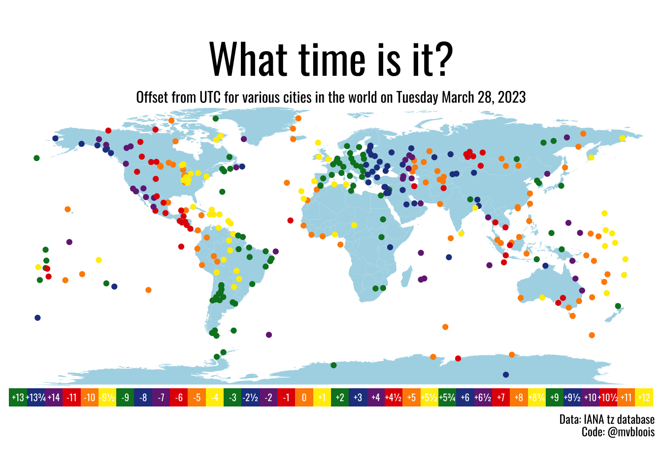 

Interesting to note the range of longitudes across some of the time zones. Additionally, there are many fewer time zones in Africa than in Europe which doesn’t align with the populations of the two continents.

praise()

[1] "You are perfect!"