library(tidyverse)
library(tidytext)
library(praise)
#devtools::install_github("ricardo-bion/ggradar", dependencies = TRUE)
library(ggradar)
library(scales)Programming Languages
The Data
The data this week comes from the Programming Language DataBase. Thanks to Jesus M. Castagnetto for the suggestion!
The PLDB has a blog with numerous articles exploring the data, such as Does every programming language have line comments?.
languages <- read_csv("languages.csv")

lang_daily <- languages %>%
  filter(pldb_id %in% c("python", "sql", "r", "stata", "spss", "sas", #"latex", "markdown",
                        "matlab", "mathematica"))
lang_daily %>%
ggplot(aes(x = appeared, y = isbndb)) +
geom_point() +
geom_text(aes(label = pldb_id), vjust = 1.5)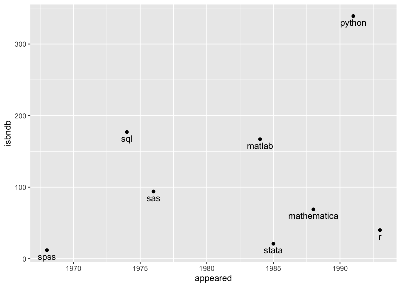
Consider the following variables that we might want to compare across some standard programming languages used around here.
lang_daily %>%
  select(pldb_id, appeared, number_of_jobs, number_of_users, book_count, language_rank)
# A tibble: 8 × 6
pldb_id appeared number_of_jobs number_of_users book_count language_rank
<chr> <dbl> <dbl> <dbl> <dbl> <dbl>
1 python 1991 46976 2818037 342 3
2 sql 1974 219617 7179119 182 4
3 matlab 1984 32228 2661579 177 10
4 r 1993 14173 1075613 40 15
5 sas 1976 4682 361103 96 35
6 mathematica 1988 1553 148741 72 44
7 spss 1968 9587 965674 14 103
8 stata 1985 0 2816 21 241We can put the variables on the same scale by using rescale which forces each data point to be between zero and one (with the smallest value set to 0 and the largest value set to 1) using:
\[X_{rs} = \frac{X - \min}{\max - \min}\]
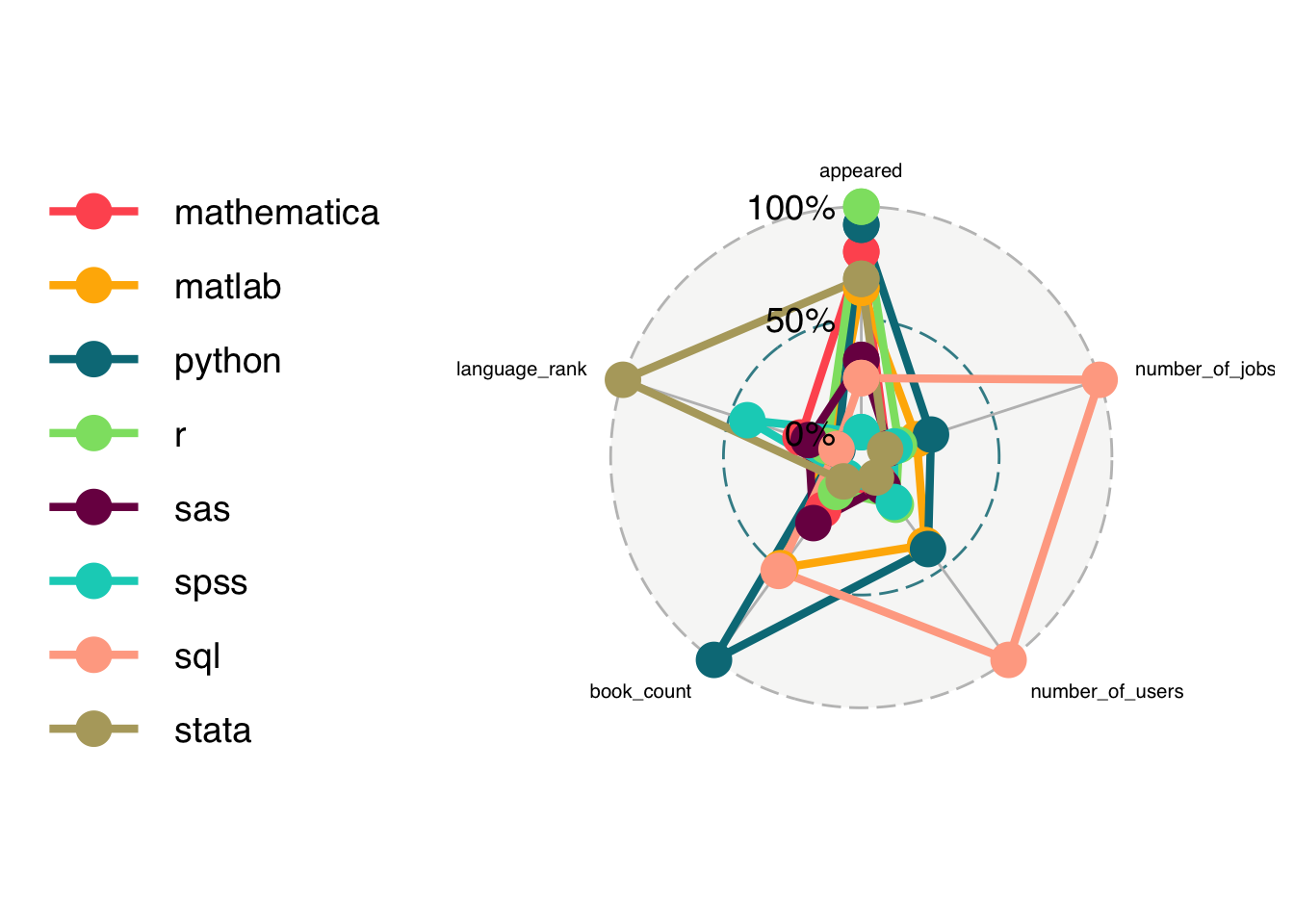
lang_daily %>%
  select(pldb_id, appeared, number_of_jobs, number_of_users, book_count,
         language_rank) %>%
  mutate_at(vars(-pldb_id), rescale) %>%
  ggradar(axis.label.size = 2.7)