Bob Ross Paintings

library(tidyverse)
library(tidytext)
library(praise)

The Data

The data this week comes from Jared Wilber’s data on Bob Ross Paintings via @frankiethull Bob Ross Colors data package.

This is data from the paintings of Bob Ross featured in the TV Show ‘The Joy of Painting’.

bob_ross <- readr::read_csv("bob_ross.csv")

hex_color <- c('#4E1500', '#000000', '#DB0000', '#8A3324', '#FFEC00', '#5F2E1F', '#CD5C5C', '#FFB800', '#000000', '#FFFFFF', '#000000', '#0C0040', '#102E3C', '#021E44', '#0A3410', '#FFFFFF', '#221B15', '#C79B00')

Grouping the paintings

I’d like to group the paintings by their titles. That is, what are the most frequent words used to describe the paintings and can we categorize them into a few groups based on those words?

top_words <- bob_ross %>%
  select(painting_title) %>%
  stringr::str_split(boundary("word")) %>%
  as.data.frame() %>%
  rename(word = `c..c....A....Walk....in....the....Woods....Mt....McKinley....Ebony...`) %>%
  mutate(word = tolower(word)) %>%
  anti_join(stop_words, by = c("word" = "word")) %>%
  table() %>%
  sort(decreasing = TRUE) %>%
  head(20) %>%
  names()

top_words_or <- paste(top_words, collapse = "|")


inword <- function(word){
  bob_ross %>%
  mutate(painting_title = tolower(painting_title)) %>%
  mutate(word_group = str_detect(painting_title, word)) %>%
  select(word_group)}

top_words %>%
  map(inword) %>%
  bind_cols() %>%
  magrittr::set_colnames(top_words) %>%
  cbind(bob_ross) %>%
  pivot_longer(cols = mountain:quiet, names_to = "word", values_to = "exist") %>%
  filter(exist) %>%  # keep only the TRUE for each word
  group_by(season, word) %>%
  summarize(across(Black_Gesso:Alizarin_Crimson, sum)) %>%
  pivot_longer(cols = Black_Gesso:Alizarin_Crimson, names_to = "paint_col",
               values_to = "count") %>%
  ggplot(aes(x = season, y = count, fill = paint_col)) + 
  geom_bar(stat = "identity") + 
  scale_fill_manual(values = hex_color) + 
  facet_wrap(~word)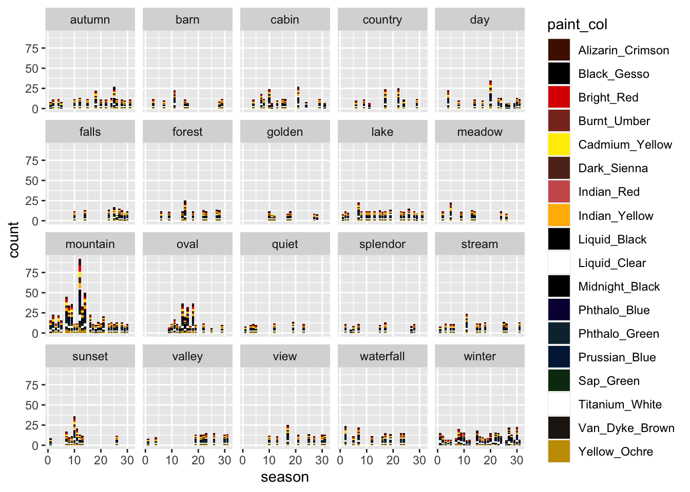

[‘Alizarin Crimson’, ‘Black Gesso’, ‘Bright Red’, ‘Burnt_Umber’, ‘Cadmium Yellow’, ‘Dark Sienna’,‘Indian_Red’, ‘Indian Yellow’, ‘Liquid Black’, ‘Liquid Clear’, ‘Midnight Black’, ‘Phthalo Blue’, ‘Phthalo Green’, ‘Prussian Blue’, ‘Sap Green’, ‘Titanium White’, ‘Van Dyke Brown’, ‘Yellow Ochre’]

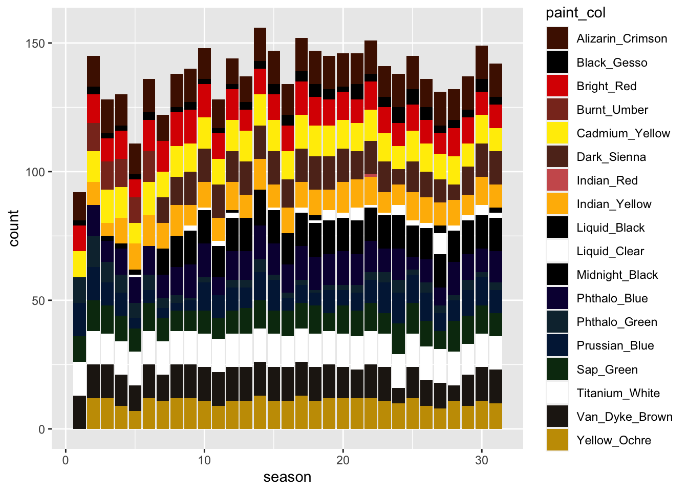
bob_ross %>%
  group_by(season) %>%
  summarize(across(Black_Gesso:Alizarin_Crimson, sum)) %>%
  pivot_longer(cols = Black_Gesso:Alizarin_Crimson, names_to = "paint_col",
               values_to = "count") %>%
  ggplot(aes(x = season, y = count, fill = paint_col)) + 
  geom_bar(stat = "identity") + 
  scale_fill_manual(values = hex_color)