Stranger Things

I want to get better at working with strings, so I’m building on the analysis by @datavizjenn. Much of the work below is taken directly from their post.

The Data

The data this week represent all of the Stranger Things dialogue and comes from 8flix.com - prepped by Dan Fellowes & Jonathan Kitt.

episodes <- read_csv("episodes.csv")
st_all_dialogue <- read_csv("stranger_things_all_dialogue.csv")

Creating dialogue to work with

st_dialogue <- st_all_dialogue |>
  tidytext::unnest_tokens(word, dialogue) |>
  filter(!is.na(word)) |>
  anti_join(stop_words, by = "word") |>
  count(season, episode, start_time, word) |> # very cool way of getting unique rows
  mutate(start_min = lubridate::minute(start_time))

Running a sentiment analysis

st_dialogue_s <- st_dialogue |>
  inner_join(get_sentiments("bing"), by = "word") |>
  group_by(season, episode, start_min, sentiment) |>
  summarize(n = sum(n)) |>
  ungroup() |>
  pivot_wider(names_from = sentiment,
              values_from = n,
              values_fill = 0) |>
  mutate(sentiment = positive - negative)

Plotting the sentiment scores

I was able to get the Stranger Things font from this blog which pointed me here.

library(sysfonts)
# Font
sysfonts::font_add_google(name = "Roboto Mono")
showtext::showtext_auto()
family <- "Roboto Mono"
sysfonts::font_add("benguiat", "BenguiatStd-Bold.otf")
showtext::showtext_auto()

# Theme Setup
font_color <- "#F2F2F2" 
title_color <- "#FF1515"
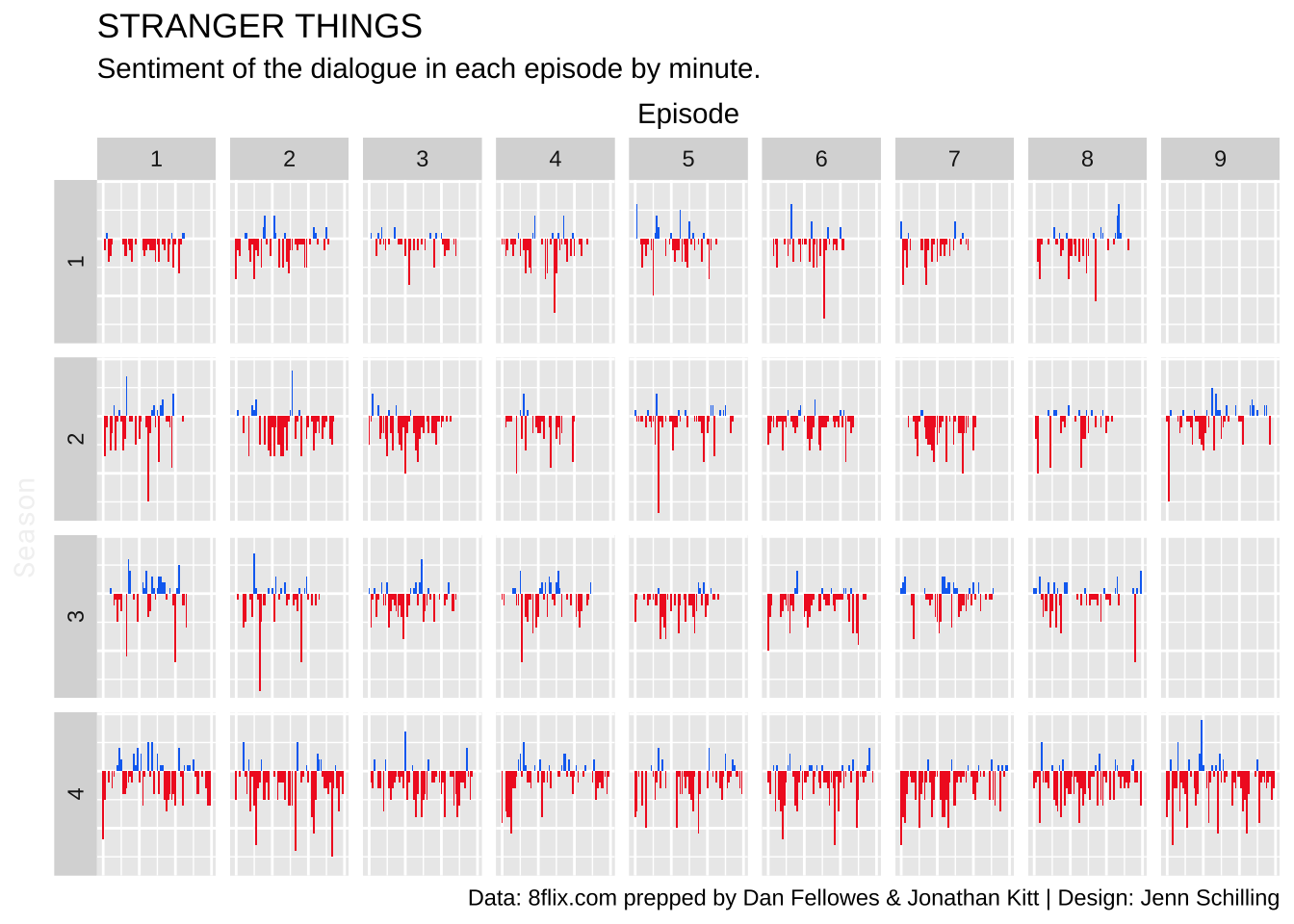
bcolor <- "#00090D"

st_dialogue_s %>%
  ggplot(aes(x = start_min, y = sentiment, fill = sentiment > 0)) + 
  geom_col() +
  facet_grid(season ~ episode, switch = "y") + 
  scale_x_continuous(position = "top") +
  scale_fill_manual(values = c("#F22727", "#0F71F2"), guide = "none") +
  labs(x = "Episode",
       y = "Season",
       title = str_to_upper("Stranger Things"),
       subtitle = "Sentiment of the dialogue in each episode by minute.",
       caption  = "Data: 8flix.com prepped by Dan Fellowes & Jonathan Kitt | Design: Jenn Schilling") +
  theme(axis.text = element_blank(),
        axis.ticks = element_blank(),
        axis.title.y = element_text(#size = 10, angle = 0, vjust = 1, hjust = 0,
                                    color = font_color, family = family),
        axis.title.x = element_text(hjust = 0, #size = 10,  
                                    color = font_color, family = family)
)

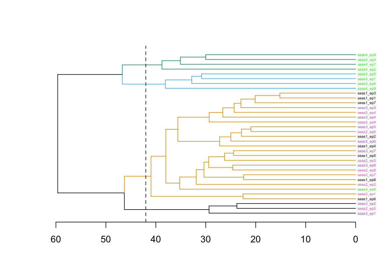
Clustering by sentiment

st_dialogue_wide <- st_dialogue_s |>
  mutate(minute = paste("min", start_min, sep = "")) |>
  pivot_wider(id_cols = season:episode,
              names_from = minute,
              values_from = sentiment,
              values_fill = 0) |>
  mutate(show = paste(paste("seas", season, sep = ""), paste("ep", episode, sep = ""), sep = "_")) 

st_dialogue_wide <- tibble::column_to_rownames(st_dialogue_wide, var = "show")

COLS <- ggthemes::colorblind_pal()(8)
pal <- c("#000000","#004949","#009292","#ff6db6","#ffb6db",
 "#490092","#006ddb","#b66dff","#6db6ff","#b6dbff",
 "#920000","#924900","#db6d00","#24ff24","#ffff6d")
# https://jacksonlab.agronomy.wisc.edu/2016/05/23/15-level-colorblind-friendly-palette/

colors <- st_dialogue_wide |>
  mutate(episode_color = case_when(
    episode == 1 ~ pal[1],
    episode == 2 ~ pal[3],
    episode == 3 ~ pal[5],
    episode == 4 ~ pal[7],
    episode == 5 ~ pal[9],
    episode == 6 ~ pal[11],
    episode == 7 ~ pal[13],
    episode == 8 ~ pal[15],
    episode == 9 ~ pal[14]
  )) |> # pull(episode_color)
  mutate(season_color = case_when(
    season == 1 ~ pal[1],
    season == 2 ~ pal[4],
    season == 3 ~ pal[8],
    season == 4 ~ pal[14])) |>
  pull(season_color)

library(dendextend)
st_dend <- st_dialogue_wide |>
  select(-season, -episode) |>
  dist() |>
  hclust(method = "ward.D") |> 
  as.dendrogram() 

dendextend::labels_colors(st_dend) <- colors[order.dendrogram(st_dend)]

st_dend |> 
  #dendextend::set("labels_col", k = 8) |>
  dendextend::set("labels_cex", .4) |>
  dendextend::set("branches_k_color", COLS, k = 4) |>
  plot(horiz = TRUE)
abline(v = 42, lty = 2)