Bigfoot

Today’s analysis is much due to Julia Silge’s screencast on chocolate ratings.

bigfoot <- read_csv("bigfoot.csv") %>%
  filter(classification != "Class C")

Tokenizing Words

Using only the Class A and Class B records, we work to build a model which can distinguish between the two types of records using the observed text column.

tidy_bf <- bigfoot %>%
  drop_na(observed) %>%
  unnest_tokens(word, observed) %>%
  filter(!word %in% stop_words$word)

tidy_bf %>%
  group_by(classification) %>%
  count(word, sort = TRUE) 

# A tibble: 40,455 × 3
# Groups:   classification [2]
   classification word         n
   <chr>          <chr>    <int>
 1 Class B        heard     5397
 2 Class A        road      3472
 3 Class B        time      2555
 4 Class A        looked    2499
 5 Class B        sound     2391
 6 Class B        night     2323
 7 Class A        time      2313
 8 Class A        feet      2284
 9 Class B        woods     2239
10 Class A        creature  2232
# … with 40,445 more rows
# ℹ Use `print(n = ...)` to see more rows

Do the words differentiate across the two classes? Maybe… hard to know from just the top 10 words in each group.

tidy_bf %>%
  group_by(classification) %>%
  count(word, sort = TRUE) %>%
  slice_max(order_by = n, n = 10) %>%
  ggplot(aes(x = n, y = word, fill = classification)) + 
  geom_bar(stat = "identity", position = position_dodge(preserve = "single"))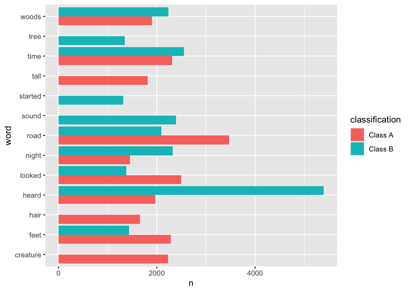

Creating model

library(tidymodels)
library(textrecipes)
set.seed(47)

bf_split <- initial_split(bigfoot)
bf_test <- testing(bf_split)
bf_train <- training(bf_split)

bf_folds <- vfold_cv(bf_train)

bf_rec <- recipe(classification ~ observed, data = bf_train) %>%
  step_tokenize(observed) %>%
  step_stopwords(observed) %>%
  step_tokenfilter(observed, max_tokens = 100) %>%
  step_tfidf(observed)

log_spec <- logistic_reg(mode = "classification") 

log_wf <- workflow(bf_rec, log_spec)

Running model

doParallel::registerDoParallel()
contrl_preds <- control_resamples(save_pred = TRUE)


log_rs <- fit_resamples(
  log_wf,
  resamples = bf_folds,
  control = contrl_preds
)

Accuracy based on the cross-validation folds:

collect_metrics(log_rs)

# A tibble: 2 × 6
  .metric  .estimator  mean     n std_err .config             
  <chr>    <chr>      <dbl> <int>   <dbl> <chr>               
1 accuracy binary     0.772    10 0.00676 Preprocessor1_Model1
2 roc_auc  binary     0.834    10 0.00825 Preprocessor1_Model1

collect_predictions(log_rs) %>%
  ggplot(aes(y = `.pred_Class A`, color =.pred_class, x = classification)) +
  geom_jitter(width = 0.5, alpha = 0.5) +
  xlab("Original class label")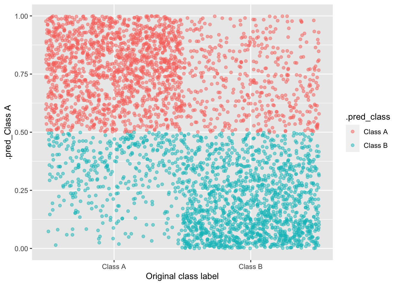

final_fitted <- last_fit(log_wf, bf_split)

extract_workflow(final_fitted) %>% tidy()

# A tibble: 101 × 5
   term                    estimate std.error statistic   p.value
   <chr>                      <dbl>     <dbl>     <dbl>     <dbl>
 1 (Intercept)               -1.00      0.352    -2.85  0.00442  
 2 tfidf_observed_10          2.55      1.85      1.38  0.168    
 3 tfidf_observed_2          -0.408     1.47     -0.278 0.781    
 4 tfidf_observed_3           3.84      1.59      2.42  0.0156   
 5 tfidf_observed_4           3.39      1.81      1.88  0.0607   
 6 tfidf_observed_across      0.520     1.59      0.328 0.743    
 7 tfidf_observed_also        4.83      1.67      2.89  0.00388  
 8 tfidf_observed_animal     -0.992     1.25     -0.796 0.426    
 9 tfidf_observed_anything    9.52      2.23      4.26  0.0000200
10 tfidf_observed_area        2.74      1.32      2.07  0.0384   
# … with 91 more rows
# ℹ Use `print(n = ...)` to see more rows

Accuracy based on the testing data:

collect_metrics(final_fitted)

# A tibble: 2 × 4
  .metric  .estimator .estimate .config             
  <chr>    <chr>          <dbl> <chr>               
1 accuracy binary         0.776 Preprocessor1_Model1
2 roc_auc  binary         0.844 Preprocessor1_Model1

Plot the words with the largest and smallest (i.e., big negative) coefficients.

extract_workflow(final_fitted) %>%
  tidy() %>%
  filter(term != "(Intercept)") %>%
  group_by(estimate > 0) %>%
  slice_max(abs(estimate), n = 10) %>%
  ungroup() %>%
  mutate(term = str_remove(term, "tfidf_observed_")) %>%
  ggplot(aes(estimate, fct_reorder(term, estimate), fill = estimate > 0)) +
  geom_col(alpha = 0.8) +
  scale_fill_discrete(labels = c("Class A", "Class B")) +
  labs(y = NULL, fill = "More from...")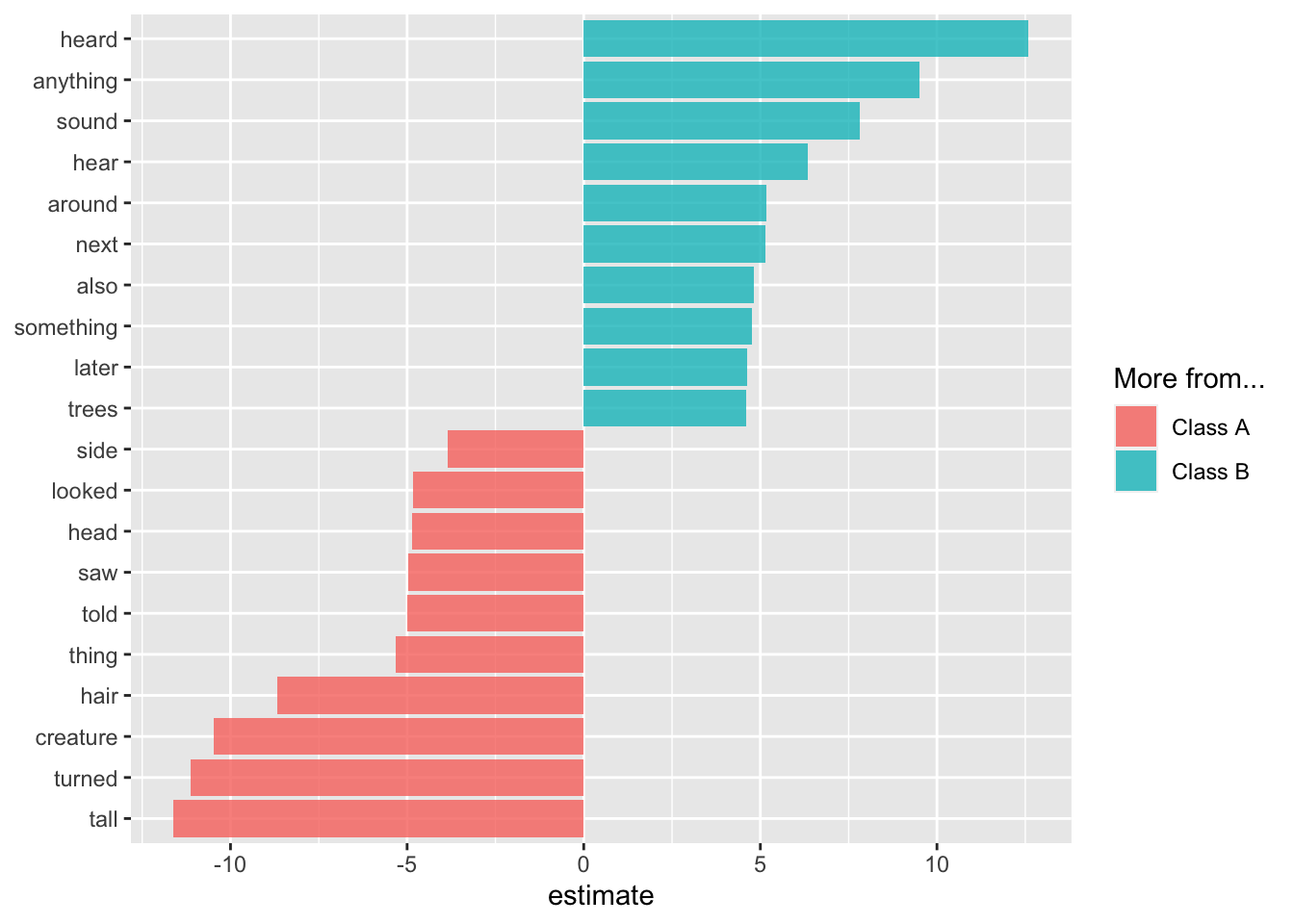

The plot aligns with the first bar plot, which showed the most common words from each class. One observation is that the Class A words are more specific (hair, tail, turned, ran, head, …) than the Class B words (anything, something, …).