Celebrating Juneteenth

Data

BlackPast.org and Vox has an article about the importance of Juneteenth as a moment and what the holiday commemorates.

BlackPast is dedicated to providing a global audience with reliable and accurate information on the history of African America and of people of African ancestry around the world. We aim to promote greater understanding through this knowledge to generate constructive change in our society.

blackpast <- read_csv("blackpast.csv") %>%
  group_by(subject) %>%
  mutate(count = n()) %>%
  ungroup() %>%
  filter(dense_rank(-count) < 6)

Events

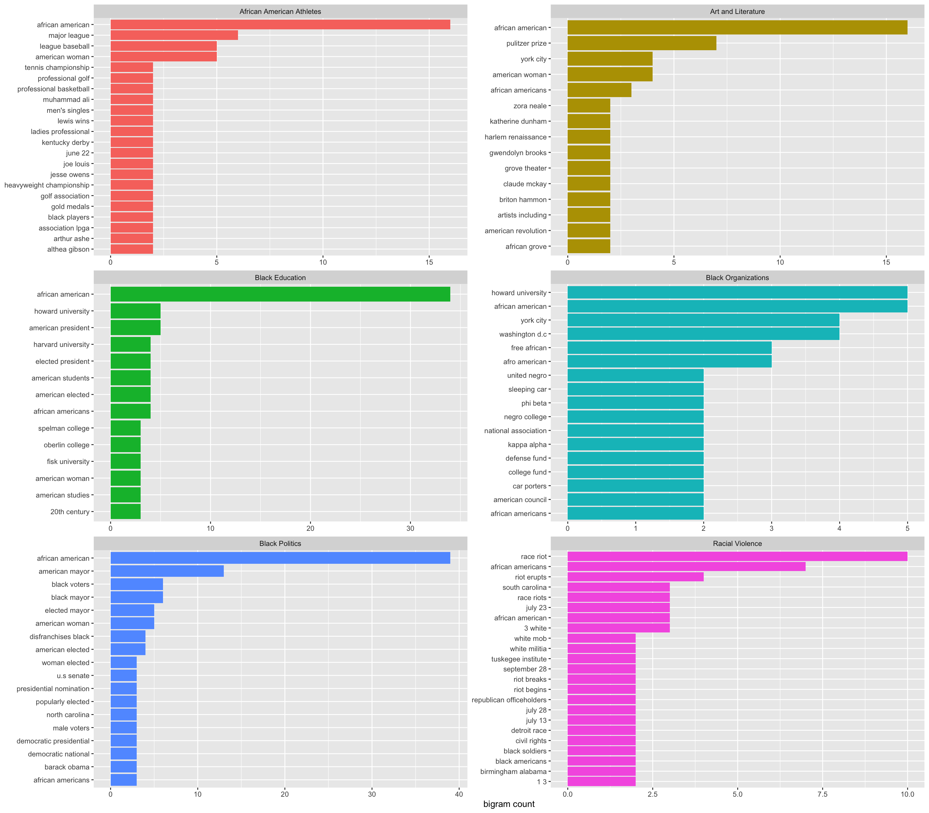
Using the tidytext, I’ll investigate bi-grams (pairs of words) in the events column of the blackpast.csv dataframe on African American and those with African ancestry around the world.

black_bigrams <- blackpast %>%
  dplyr::select(events, subject) %>%
  group_by(subject) %>%
  unnest_tokens(bigram, events, token = "ngrams", n = 2, to_lower = TRUE) 

bigrams_sep <- black_bigrams %>%
  separate(bigram, c("word1", "word2"), sep = " ")

bigrams_filtered <- bigrams_sep %>%
  dplyr::filter(!word1 %in% stop_words$word) %>%
  dplyr::filter(!word2 %in% stop_words$word)

bigram_counts <- bigrams_filtered %>%
  count(word1, word2, sort = TRUE)

bigram_counts

# A tibble: 1,870 × 4
# Groups:   subject [6]
   subject                   word1    word2         n
   <chr>                     <chr>    <chr>     <int>
 1 Black Politics            african  american     39
 2 Black Education           african  american     34
 3 African American Athletes african  american     16
 4 Art and Literature        african  american     16
 5 Black Politics            american mayor        13
 6 Racial Violence           race     riot         10
 7 Art and Literature        pulitzer prize         7
 8 Racial Violence           african  americans     7
 9 African American Athletes major    league        6
10 Black Politics            black    mayor         6
# … with 1,860 more rows

bigrams_united <- bigrams_filtered %>%
  unite(bigram, word1, word2, sep = " ")

sorted_bigrams <- bigrams_united %>%
  count(subject, bigram, sort = TRUE) %>%
  top_n(10) %>%
  group_by(subject) %>%
  arrange(subject, n) %>%
  unite("subj_bigram", subject, bigram, sep = "_", remove = FALSE) %>%
  data.frame() %>%
  mutate(subj_bigram = factor(subj_bigram, levels = subj_bigram))
  
sorted_bigrams %>%  
  group_by(subject) %>%
  ggplot(aes(x = subj_bigram, y = n, fill = subject)) + 
  geom_col(show.legend = FALSE) + 
  labs(x = NULL, y = "bigram count") + 
  coord_flip() + 
  scale_x_discrete(breaks = sorted_bigrams$subj_bigram,
                   labels = sorted_bigrams$bigram ) + 
  facet_wrap(~subject, ncol = 2, scales = "free") 

Bar plots showing bigram tendencies across the events with the most instances. Unsurprisingly “African American” is a common bigram for most of the event types.